Past exam of the mathematics course of the year 1 of the natural sciences course of the University of Cambridge / 2018 / Paper 2

The direction vectors are $\mathbf{u}=(1,-2,1)$ and $\mathbf{v}=(0,-2,1)$. Their cross product is $(0,-1,-2)$, with norm $\sqrt{5}$. A unit normal to the plane is thereforeThe two intersecting directions span the plane, so a vector orthogonal to both is a normal vector to that plane.

The plane contains $(1,0,1)$ and has normal vector $(0,1,2)$, so its equation is $y+2z=2$. In the equation $\mathbf{n}\cdot \mathbf{r}=d$ with a unit normal, $|d|$ is the perpendicular distance from the origin. Consequently

The exponential definition of hyperbolic sine gives $e^z-e^{-z}=0$, or $e^{2z}=1$. Taking every branch of the complex logarithm givesFor hyperbolic cosine, multiply $\cosh z+1=0$ by $2e^z$ to obtain $(e^z+1{)}^2=0$. Thus $e^z=-1$, giving

The vectors $(1,1{)}^{\mathsf{T}}$ and $(1,-1{)}^{\mathsf{T}}$ are eigenvectors: multiplication adds or subtracts the two entries in a row. Their eigenvalues are thereforeThe second eigenvalue may be positive, zero or negative as the real parameter changes.

Multiply the Maclaurin series $\ln (1+x^2)=x^2-x^4/2+O(x^6)$ and the geometric series $(1+x^2{)}^{-1}=1-x^2+O(x^4)$. The first two nonzero terms are

To distinguish the one-variable profile from the resulting two-variable function, write $u(x,t)=F(\xi )$ with $\xi =x{e}^{-t}$. The chain rule gives $u_t=-x{e}^{-t}{F}^{\prime }(\xi )$ and $u_x=e^{-t}{F}^{\prime }(\xi )$, so $u_t+x{u}_x=0$. Thus any differentiable profile of $x{e}^{-t}$ solves the partial differential equation.

The initial condition selects $F(\xi )=\ln \xi$ on the positive half-line. HenceThis satisfies both the partial differential equation and the given data at $t=0$.

For $r>0$, the partial derivatives of radius are $r_x=x/r$, $r_y=y/r$ and $r_z=z/r$. Applying the chain rule to the outer sine and then the radial profile gives the Cartesian coordinates of the gradient:At the origin these coordinate formulas require a differentiable radial extension; differentiability of $f$ as a one-variable profile alone does not guarantee it.

The vector field has only a vertical component, namely $f(r)$. Its divergence is therefore its vertical partial derivative:

The integrating factor for this linear ordinary differential equation is $e^x$. Multiplication gives $(e^{x}y{)}^{\prime }=1$, so $e^{x}y=x+C$. The initial condition sets $C=0$, giving

Near the initial condition $y=1$, divide by $y^2$ and separate variables: $y^{-2}dy=-x^{2}dx$. Integration gives $-1/y=-x^3/3+C$; the initial value fixes $C=-1$. Thus the solution of the separable differential equation isThe stated interval is the maximal connected interval containing zero: the solution diverges at its left endpoint. The constant solution $y=0$ does not satisfy the initial condition.

The vector field is radial, while the differential displacement along a centred circle is tangential. These directions are orthogonal, so the dot product vanishes at every point. Hence

Use the outward unit normal on the unit sphere and the convention that $\theta$ is measured from the positive vertical axis. Then $\mathbf{F}\cdot \mathbf{n}=\sin \theta$, while the spherical coordinates area element is $dS=\sin \theta d\theta d\varphi$. The flux is therefore

The gradient components areAway from the vertical axis, $x\ne 0$, so $u_y=0$ forces $y=0$. The other stationary point equation then gives $x^2=3/2$. Therefore the two requested points areEvery point with $x=0$ also has zero gradient, but those points are explicitly excluded.

Normalization of the probability density function requires $1=\alpha {\int }_0^{\pi }\sin xdx=2\alpha$. Thus

The expected value follows by integration by parts:The same result follows from symmetry of the probability density function about $\pi /2$.

Let $\Delta =[\mathbf{a},\mathbf{b},\mathbf{c}]\ne 0$. These three vectors are linearly independent, so write $\mathbf{d}=\alpha \mathbf{a}+\beta \mathbf{b}+\gamma \mathbf{c}$. Taking the dot product with $\mathbf{b}\times \mathbf{c}$ gives $\alpha =[\mathbf{b},\mathbf{c},\mathbf{d}]/\Delta$. Likewise, the dot products with $\mathbf{c}\times \mathbf{a}$ and $\mathbf{a}\times \mathbf{b}$ giveHere the cyclic invariance and sign change under an interchange of the scalar triple product fix every sign. Substituting the three coefficients provesThis is precisely coordinate extraction using the reciprocal basis $(\mathbf{b}\times \mathbf{c},\mathbf{c}\times \mathbf{a},\mathbf{a}\times \mathbf{b})/\Delta$.

Put $\mathbf{v}={\mathbf{r}}_0-\mathbf{a}$. The squared distance to a point on the line is $|\mathbf{v}-\lambda \hat{\mathbf{t}}{|}^2$. Since $|\hat{\mathbf{t}}|=1$, completing the square in $\lambda$ gives its minimum at $\lambda =\hat{\mathbf{t}}\cdot \mathbf{v}$, with value $|\mathbf{v}{|}^2-(\hat{\mathbf{t}}\cdot \mathbf{v}{)}^2$. The cross product identity $|\hat{\mathbf{t}}\times \mathbf{v}{|}^2=|\mathbf{v}{|}^2-(\hat{\mathbf{t}}\cdot \mathbf{v}{)}^2$ therefore provesFor the given line, $\hat{\mathbf{t}}=(1,1,0)/\sqrt{2}$, so its squared distance to $(x,y,z)$ is $(x-y{)}^2/2+z^2$. Substituting the parabola givesThe global minimum occurs at $\mu =\pm 1$, henceThe corresponding points on the parabola are $\pm (1,1+2\sqrt{3},0)+(0,0,-3)$; their nearest points on the line are $\pm (1+\sqrt{3},1+\sqrt{3},0)$. The connecting vectors are orthogonal to the line, as the projection calculation requires.

Write $s=\hat{\mathbf{n}}\cdot \mathbf{x}$. Taking the dot product of the equation with the unit vector $\hat{\mathbf{n}}$ gives $2s+s^2=-1$, so $(s+1{)}^2=0$ and $s=-1$.

Now take the cross product with $\hat{\mathbf{n}}$. The vector triple product gives $\hat{\mathbf{n}}\times (\hat{\mathbf{n}}\times \mathbf{x})=s\hat{\mathbf{n}}-\mathbf{x}=-\hat{\mathbf{n}}-\mathbf{x}$, soThe original equation, now with $s^2=1$, also gives $\hat{\mathbf{n}}\times \mathbf{x}=\mathbf{b}-\hat{\mathbf{n}}-2\mathbf{x}$. Substitution eliminates the remaining cross product of the unknown and yieldsIts dot product with $\hat{\mathbf{n}}$ is $-1$, and direct substitution using the vector triple product verifies the original equation. The elimination gives a unique solution without choosing components. It is also an application of the inverse of a scalar plus a cross-product operator after the scalar component has been fixed.

For $r>0$, differentiate $r=\sqrt{x^2+y^2}$ while keeping the other coordinate fixed in the Cartesian coordinate system:The origin is excluded from this polar coordinates chart.

Differentiate the angular relation locally, or use $d\varphi =(xdy-ydx)/(x^2+y^2)$. Holding each other coordinate fixed givesThese are local partial derivatives on a consistent angular branch, independent of where its branch cut is placed.

Apply the multivariable chain rule to $f(x,y)=g(r(x,y),\varphi (x,y))$. Using the coordinate partial derivatives above givesEquivalently, ${\partial }_x=\cos \varphi {\partial }_r-(\sin \varphi /r){\partial }_{\varphi }$ and ${\partial }_y=\sin \varphi {\partial }_r+(\cos \varphi /r){\partial }_{\varphi }$. Their coefficients vary with position and must also be differentiated when applying them twice.

Write $c=\cos \varphi$ and $s=\sin \varphi$. The needed coefficient derivatives are $c_x=s^2/r$, $s_x=-sc/r$, $c_y=-sc/r$ and $s_y=c^2/r$. Apply the product rule to both terms of $f_x=c{g}_r-(s/r)g_{\varphi }$ and use the chain rule for the derivatives of $g$. Collecting terms givesSimilarly, differentiating $f_y=s{g}_r+(c/r)g_{\varphi }$ givesOn addition, both the mixed partial derivative terms and the first angular derivative terms cancel. Using $s^2+c^2=1$, the Laplacian in polar coordinates is

The double-angle formula gives $r^2\sin 2\varphi =2(r\cos \varphi )(r\sin \varphi )=2xy$. Therefore

In the positive quadrant, both components of the gradient are positive. Along $y=x$ the arrows point along $(1,1)$; near the horizontal axis they point mainly upwards, and near the vertical axis mainly rightwards. The level sets are the hyperbolas $xy=f/2$, including the coordinate axes for level zero. The gradient is orthogonal to each regular level set and points towards increasing values of $f$.

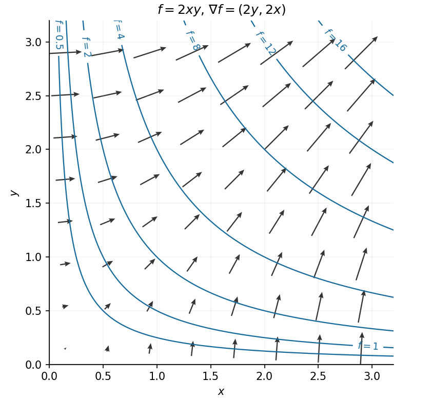
At $(1,2)$, the gradient is $(4,2)$. The requested direction must be normalized to the unit vector $(1,1)/\sqrt{2}$. The directional derivative is thereforeUsing $(1,1)$ without normalization would instead measure change per unit of a differently scaled path parameter.

The field $\mathbf{F}$ is not a conservative vector field: either nonzero closed line integral computed below rules out a scalar potential. Equivalently, its planar curl is ${\partial }_x{F}_y-{\partial }_y{F}_x=1-(-1)=2$.

For $\mathbf{G}$, integrating ${\Phi }_x=2x{y}^2$ gives $\Phi =x^2{y}^2+h(y)$. Matching ${\Phi }_y=2y{x}^2$ then gives $h^{\prime }=0$. ThusThis also explains why both closed line integrals of $\mathbf{G}$ vanish.

Starting at $(1,0)$, traverse the right, top, left and bottom sides in that order. For $\mathbf{F}$, the differential expression is $-ydx+xdy$. The four line integral contributions are respectively $1,1,0,0$, so the total is two.

For $\mathbf{G}$, the expression is $2x{y}^{2}dx+2y{x}^{2}dy$. The right side contributes ${\int }_0^{1}2ydy=1$, and the top side contributes ${\int }_1^{0}2xdx=-1$; the other sides contribute zero. Therefore

Parametrize the circle by $\mathbf{r}(t)=(\cos t,\sin t)$, $0\le t\le 2\pi$. Its tangent is ${\mathbf{r}}^{\prime }=(-\sin t,\cos t)=\mathbf{F}(\mathbf{r}(t))$, so the dot product $\mathbf{F}\cdot {\mathbf{r}}^{\prime }$ is one. For the other field,Integrating around the full circle gives

Substituting the endpoint parameter values givesThe curve lies on the unit circular cylinder $x^2+y^2=1$. Its azimuth increases from zero to $\pi /2$ while its height increases linearly, so it is one quarter-turn of a rising helix. The arrow in the sketch indicates increasing parameter.

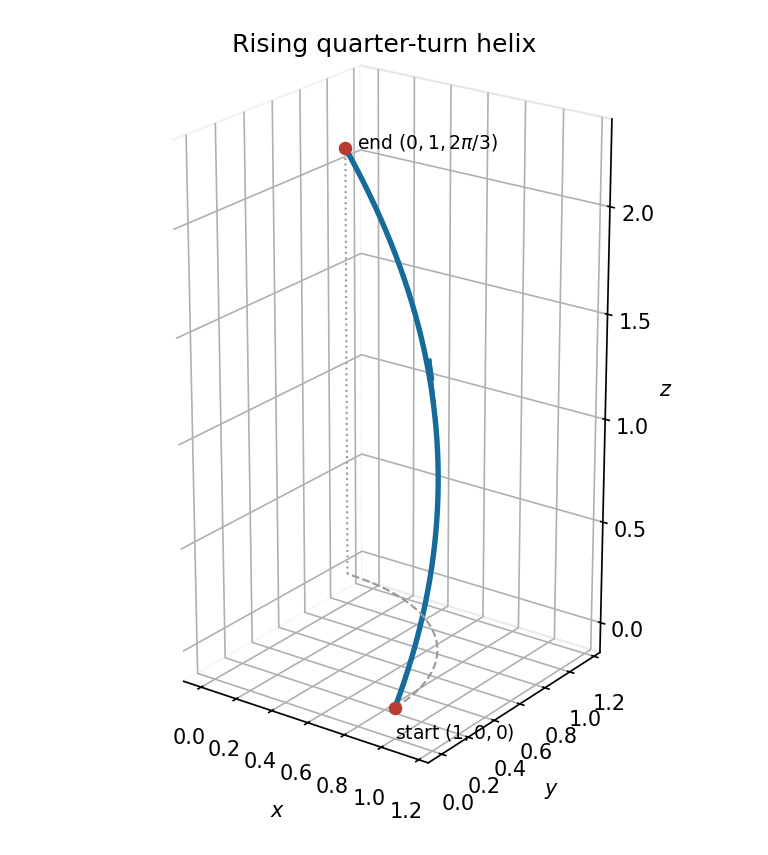
The arc length factor is the norm of the tangent:Hence $ds=10dt$ and $\Phi =xy=\cos 6t\sin 6t=\frac{1}{2}\sin 12t$. The scalar line integral is thereforeThis uses scalar arc length, rather than the oriented displacement used in the vector line integrals of part (a).

Distinguish the production type as well as the stopping position. The sample space has the six outcomesHere $x_k$ in an event means $X=x_k$. Their joint probabilities are $p{g}_k$ and $(1-p)d_k$, respectively. The conditional stopping laws obey ${\sum }_{k=0}^2{g}_k={\sum }_{k=0}^2{d}_k=1$; with the stated strict positivity all six outcomes are possible.

Multiply the production probability by the conditional stopping probability:

The good and defective cases are disjoint and exhaustive. The law of total probability therefore gives

Divide the relevant joint probability by the marginal stopping probability. By Bayes' theorem,The denominator is positive under the stated assumptions.

The condition $X>x_0$ selects positions $x_1$ and $x_2$. Their combined good-ball joint probability is $p(g_1+g_2)$, and their total probability is $p(g_1+g_2)+(1-p)(d_1+d_2)$. Thus

For $0\le k\le n$, sum the marginal stopping probabilities over the selected tail:Equivalently it is $p(1-{\sum }_{j=0}^k{g}_j)+(1-p)(1-{\sum }_{j=0}^k{d}_j)$. At $k=n$, both empty tail sums are zero, as required.

The event includes stopping positions zero through $k$. Applying Bayes' theorem to their joint and marginal probabilities givesThis conditional probability is defined whenever its conditioning event has positive probability. At $k=n$, it reduces to $p$.

There are $99$ possible stopping points, so the equal defective-ball probabilities are $d_k=1/99$. With $g_0>0$, the desired conditional probability givesThus, for a fixed good-ball stopping law,Since $g_0\le 1$, the smallest possible production probability over admissible stopping laws isIf strict positivity of every $g_k$ is additionally imposed in this general case, then $g_0<1$ and one only has the infimum $1/2$, approached as $g_0\to 1$. The paper states that strict-positivity assumption explicitly for part (a), not for the general case in part (b). Without choosing or bounding $g_0$, the exact fixed-law answer remains $1/(1+g_0)$.

For the homogeneous linear differential equation, the characteristic equation is $r^2-2r+2=0$, with polynomial roots $1\pm i$. Its homogeneous solution is therefore $e^x(A\cos x+B\sin x)$.

Use the method of undetermined coefficients for a particular solution $y_p=a{x}^2+bx+c$. Substitution givesEquating coefficients yields $a=1$, $b=2$ and $c=1$. Hence the general solution is

The characteristic polynomial factors as $(r+1)(r+2)$, so the homogeneous solution is $A{e}^{-x}+B{e}^{-2x}$. The forcing $e^{-x}$ already occurs in that solution, so a constant multiple of $e^{-x}$ cannot be a particular solution. Use $y_p=Cx{e}^{-x}$ instead. Its derivatives are $C(1-x)e^{-x}$ and $C(x-2)e^{-x}$, so substitution gives $C{e}^{-x}$ and fixes $C=1$. ThusThe extra factor of $x$ accounts for the repeated forcing exponent in the method of undetermined coefficients.

Under $y=xu$, the product rule gives $y^{\prime }=u+x{u}^{\prime }$ and $y^{\prime \prime }=2u^{\prime }+x{u}^{\prime \prime }$. Substitute these into the original equation:Since $x>0$, this is precisely $x{u}^{\prime \prime }+u^{\prime }=0$, or $(x{u}^{\prime }{)}^{\prime }=0$. Integrating twice gives $x{u}^{\prime }=C_1$ and $u=C_1\ln x+C_2$. ThereforeThe two independent solutions of a differential equation supply the general solution of this second-order linear ordinary differential equation.