Take the base-ten logarithm of both positive sides. The exponentiation rule for logarithms gives , hence
Move the constant term to the left and factor the cubic polynomial:Setting each factor to zero gives all three polynomial roots:
The quadratic formula gives the two polynomial roots . Its leading coefficient is positive, so the quadratic polynomial is strictly negative between them. Therefore
Matching the two parametric equations at an intersection gives and . The Pythagorean trigonometric identity therefore requiresFor , the sine is one and the cosine is zero; for , the cosine is one and the sine is zero. Keeping the stated half-open angular interval givesThe corresponding points are and ; both satisfy the original parametric equations.
The two labelled regions in the original diagram are complementary circular sectors. Their areas add to and satisfy , so . The sector with central angle has area . Hence
The two radii enclose the angle , so the triangle has area . From the sector calculation, . Consequently
A space diagonal of the unit cube has displacement vector . Its Euclidean norm, or two successive applications of the Pythagorean theorem, givesThe requested diagonal joins opposite vertices; would be the diagonal of a face.
Choose two distinct space-diagonal directions and . Their dot product is one and their norms are both . Thus the acute angle between their unoriented lines isAny two distinct space diagonals have an absolute dot product of one when represented with components , so they give the same acute angle.
The binomial theorem givesThus, to three decimal places,The first three nonconstant terms already determine this rounding; the remaining positive terms total less than .
The initial term at is three, and the common ratio is . The convergent geometric series therefore sums to
The product rule gives . The exponential function never vanishes, so a stationary point requires . In the given interval this means . Substitution givesThe derivative changes from positive to negative there, making it a strict local maximum.
In the completed-square equation, the right side is the squared radius of the circle. Taking its positive square root gives
The two derivatives are and , both equal to six at . Their common tangent line through is , or . Setting gives its intersection with the vertical axis:
The factor has modulus and principal argument . Multiplication by adds to its complex argument, while the real factor halves its modulus. HenceTaking the principal logarithm for givesThis complex number lies in the second quadrant. Its modulus follows from the sum of squared components, and its principal argument follows by the second-quadrant correction:All arguments of this fixed add integer multiples of to the displayed one.
If is interpreted as the multivalued complex logarithm, there is instead a family , where and . Then , and the principal argument is for , or for . This records the logarithm-branch choice that the paper leaves implicit.
Using the exponential definition of hyperbolic tangent, set :Here , so the resulting points are not poles. Taking all values of the complex logarithm gives . ThusEquivalently , so these are exactly the imaginary-axis solutions of .
By De Moivre's theorem, is the real part of . Writing and , the binomial theorem givesUse the Pythagorean trigonometric identity and expand:Therefore
The region is an unbounded wedge in the first quadrant, lying between the rays and . Both boundaries and the origin are included. For integration in the opposite order, the same region is with .
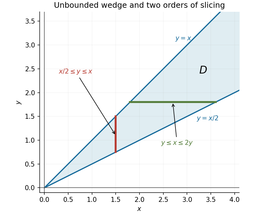
The integration wedge and representative vertical and horizontal slices
. Details. For fixed , integrate first over :The integrand is nonnegative, so this order of the double integral is legitimate even before its finiteness is known. Applying the scaled Gaussian integral yields
Reverse the order in the nonnegative double integral, using and . For , an antiderivative in is . ThusLet denote the requested improper integral. Its numerator is near zero, so its apparent singularity is removable; it also decays at infinity. We may therefore separate the preceding expression into the convergent integralsIt follows thatThe two terms divided separately by would each have a divergent integral at zero; the cancellation in their difference is essential.
Scale the ellipsoid to a unit ball usingwith , and . This is spherical coordinates followed by a diagonal linear transformation, so the Jacobian determinant is . The required volume integral is
The ellipsoid and the exponential factor are invariant under separate reflections of any coordinate. Split the integrand into its two polynomial terms. The term times that exponential is odd in , so its volume integral vanishes by reflecting . The other term times the exponential is odd in , so its volume integral vanishes by reflecting . Both integrands are continuous on a bounded region. Therefore odd-integrand cancellation by reflection gives
For , divide by to obtain , a first-order linear ordinary differential equation. An integrating factor is on either interval not crossing zero, since the product rule givesIntegration and division by give the explicit general solutionThe original equation would read at zero, so no solution can include that point.
Rewrite the linear ordinary differential equation as . Multiplication by its integrating factor gives . Integrating yieldsThe general solution consists of this particular solution and the homogeneous solution .
The original PDF has in the denominator and on the left. Rearrange it into the differential formThe cross partial derivatives of its coefficients are both four, so it is an exact differential form. Integrating its first coefficient in gives a potential . Matching gives . Therefore an implicit general solution isDifferentiating verifies . A solution graph is understood only on intervals where its denominator is nonzero; the printed quotient does not define a derivative when .
For real solutions with , the square root requires . First retain the solution , which would be lost by dividing by a square root of .
For , use the homogeneous first-order differential equation substitution , so , and . The equation becomesThis is now a separable differential equation. Integration gives . Since , the positive solutions satisfyThe implicit family is sufficient here because only parts (a) and (b) request an explicit expression. It also shows why the nonnegative choice of matters: denotes the positive square root.
The exponential function is strictly positive, so the zero level set is determined entirely by its prefactor:This is a rectangular hyperbola with branches in the first and third quadrants.
The sign of is the sign of . ThereforeThe positive region includes both coordinate axes, the second and fourth quadrants, and the portions of the first and third quadrants on the origin side of the hyperbola. The two negative regions lie beyond its branches. The left-hand panel shows these regions; its markers locate the stationary points calculated next.
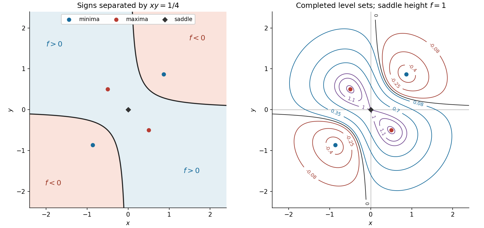


Set both components of the gradient to zero. After dividing out the nonzero exponential, they are equivalent toAdding and subtracting gives and . If , the first equation reduces to , giving the origin and the two diagonal points. If , it reduces to , giving the origin and the two opposite-diagonal points. The alternative simultaneous values and are incompatible, so these cases exhaust the possibilities. Thus the five stationary points areThey are marked in both panels of the figure.
Evaluate the Hessian matrix at the five stationary points. At the origin it iswhose eigenvalues are and , so the origin is a saddle point. At the two points with ,whose eigenvalues are and . Both are positive, so these are strict local minima. At the two points with ,whose eigenvalues are and . Both are negative, so these are strict local maxima. In summary,The quadratic changes along the orthogonal directions and also provide a direct justification of these classifications.
The completed contour plot is shown in the right-hand panel. Its geometry follows from the symmetries and , together with as . For orientation, the two local minima have value , the two local maxima have value , and the saddle point has value one.
Negative level sets between and zero form separate closed curves around the two local minima in the first and third quadrants. Positive level sets below one form a single closed curve enclosing the origin and both local maxima. At level one, a critical level set crosses itself at the origin and surrounds the two local maxima in two lobes. Between one and , the level sets split into separate closed curves around those local maxima. The zero level set remains the two unbounded branches .
Near the origin, the Taylor expansion is . Consequently the crossing directions at the saddle height satisfy , giving the local shape of the critical level set.
The first terms of Taylor's theorem, with the Taylor remainder in mean-value form, arewhere lies between and for . Sufficient hypotheses are continuous derivatives through order on the interval between the endpoints and an th derivative in its interior. At the remainder is zero. The finite Taylor polynomial ends at degree ; this identity does not require convergence of an infinite Taylor series.
Since , write and multiply the two power series. Equating coefficients with the identity givesSolving successively yieldsThese are the constant, linear and quadratic terms; particular coefficients may vanish. For a convergent power series defining near zero, continuity and ensure its reciprocal is also defined in a neighborhood of zero.
Multiply the Maclaurin series of hyperbolic cosine by the binomial series for the reciprocal square root:The quadratic terms cancel, while the quartic coefficient is . HenceThe absence of odd powers follows from the function's even symmetry.
Combine the logarithms first and factor out the limiting constant:Apply the Taylor expansion with . The first three nonzero terms, including the constant, areThis is an asymptotic expansion in reciprocal powers of .
The slope of the particle's straight trajectory is , soThe endpoint directions are parallel to the screen and do not give finite collisions, but each has zero probability in the continuous angular model. The relation therefore holds almost surely.
The angular interval has width , so its continuous uniform distribution has probability density functionIntegrating this probability density function gives the cumulative distribution functionValues of the probability density function at the two individual endpoints may be assigned arbitrarily without changing any probability.
Articles were limited to the first 100 out of 291 total.
Articles by others on the same topic
There are currently no matching articles.