For a continuously differentiable vector field on a bounded volume with piecewise smooth closed boundary , the divergence theorem stateswhere is the outward unit normal vector. Thus total outward flux through a closed surface equals the integral of the local divergence inside it. A nonclosed surface first needs a suitable closure, with the added surface's flux accounted for separately.
In cylindrical coordinates, the surface has radius . It is the lateral surface of a right circular cone, with vertex at the origin and axis along positive . Its height is and the limiting upper rim has radius ; the horizontal disk at that rim is absent. The half-angle from the vertical satisfiesThe upper rim is excluded by , which does not affect any convergent surface integral. The vertex likewise contributes no area.
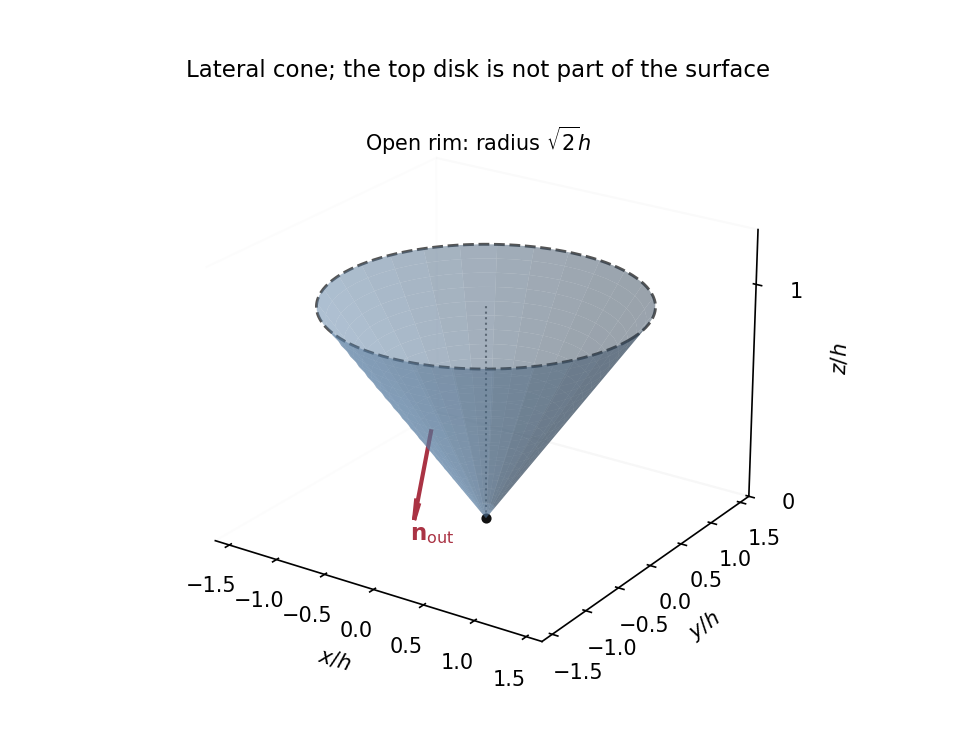
The open lateral cone and its auxiliary closing cap
. Original sketch in units of . The dashed upper rim bounds an auxiliary disk used only to apply the divergence theorem. The arrow shows the outward lateral normal, which has a downward component. Details.
Close the cone with the horizontal disk at height , and let be the enclosed solid. The divergence isThe term integrates to zero by reflection symmetry of each circular cross-section. Using the divergence theorem and cylindrical coordinates, the closed-surface flux isThe outward normal on is , so its flux is its area times :Subtracting this cap contribution gives the required lateral flux:This is conical flux by closing with a cap. The normal convention matters: on the lateral cone the outward normal points radially outwards and partly downwards, so the contribution to the lateral flux is negative. To justify applying the theorem at the vertex, truncate a small tip and take its size to zero; the extra flux vanishes because is regular there.
For , the derivatives areSubstitution cancels the two terms , giving the diffusion equationThis is a scalar integrating factor for a reaction-diffusion equation, since up to a constant. We use , so the factor never vanishes. A classical solution at the initial corners additionally requires compatible data, and .
The transformed endpoint values are and . Apply boundary lifting with . The lifted profile is linear, so with homogeneous Dirichlet boundary conditions andFor separation of variables, put . Then . The endpoint conditions give nonzero spatial modes only for , , with and . Henceby orthogonality of the sine modes. Only the mode is present. Undoing both substitutions givesAt this has the prescribed initial profile, and at it is . Differentiating also verifies the original evolution equation directly.
The nonstationary part of decays exponentially, whereas the integrating factor grows quadratically. For fixed ,ConsequentlyAt , both expressions are identically zero; the ratio formulation is understood for . The diffusion modes have died away, leaving the lifted linear profile multiplied by the reaction-induced amplitude factor.
A causal Green function vanishes before the impulse. For it solves the homogeneous linear ordinary differential equation, whose characteristic roots are . Thus it has the formContinuity at is necessary to avoid a delta derivative in , so . Integrating its forced equation across the impulse gives the jump condition for an impulse, . The derivative from below is zero and the derivative from above is , givingHere is the Heaviside step function. The zero initial data exclude any additional homogeneous response. By the superposition principle, the output for a general locally integrable input isThe upper endpoint causes no unwanted term in the first derivative because ; in the second derivative its unit derivative jump reproduces the input.
The pulse height is the constant , not the time variable. In the undamped case the convolution therefore reduces toIntegration gives the continuous displacement and velocityThe post-pulse expression is equivalently . Since , it vanishes for every subsequent time precisely when . ThusThese are integer multiples of the oscillator's natural period . At such switch-off times both and are zero. Vanishing displacement alone would not suffice: a nonzero switch-off velocity would restart an oscillation. This is rectangular-pulse cancellation of an undamped oscillator.
For the stated forward Fourier transform, the inverse has the opposite exponential sign and a factor :This holds under the usual hypotheses for Fourier inversion, or in the sense of distributions when appropriate.
Suppose initially that are absolutely integrable, so Fubini's theorem justifies exchanging the integrations. The transform of their convolution isSet , so and . The exponential separates:Therefore the convolution theorem isNo extra occurs in this direction with the specified normalization.
Since , the causal damped sine has an absolutely convergent Fourier transform for real . Resolving the sine into complex exponentials givesCombining the two fractions yieldsThe formula also includes , for which both the original function and its transform vanish. Its sign reverses when the real parameter reverses.
For an integrable applied voltage, the convolution theorem givesThe integrated electric current is the zero-frequency transform, . Since can be arbitrary, zero total electric charge for every such input is equivalent toFor nonzero , this can be writtenBecause both amplitudes are positive, nonzero must have opposite signs. If exactly one is zero there is no cancellation with positive amplitudes; if both vanish the kernel is identically zero and any amplitudes work. In particular, if both frequency parameters were additionally required to be positive, no such nontrivial system would exist. The PDF requires positivity of , but allows real fixed .
This is zero-frequency cancellation of a causal response kernel. The phrase arbitrary voltage is understood within a class for which the net-charge integrals exist; a permanent DC input need not have finite total charge.
An matrix is diagonalizable over a chosen field exactly when it has a basis of linearly independent eigenvectors. Equivalently, is diagonal for some invertible . Distinct eigenvalues suffice but are not necessary. For example,is not diagonalizable: its only eigenvalue is and its eigenspace is the one-dimensional span of . It is a nontrivial Jordan block.
A Hermitian matrix satisfies , where the dagger denotes conjugate transpose. If with , thenThe denominator is positive real, soFor and , Hermiticity also givesThusThis is the necessary qualification to the PDF's orthogonality wording: arbitrary eigenvectors belonging to a repeated eigenvalue need not be orthogonal. Within each repeated eigenspace, Gram-Schmidt orthogonalization produces an orthonormal basis; together the eigenspaces give an orthonormal eigenbasis by the finite-dimensional spectral theorem. For example, and are nonorthogonal eigenvectors of the identity matrix.
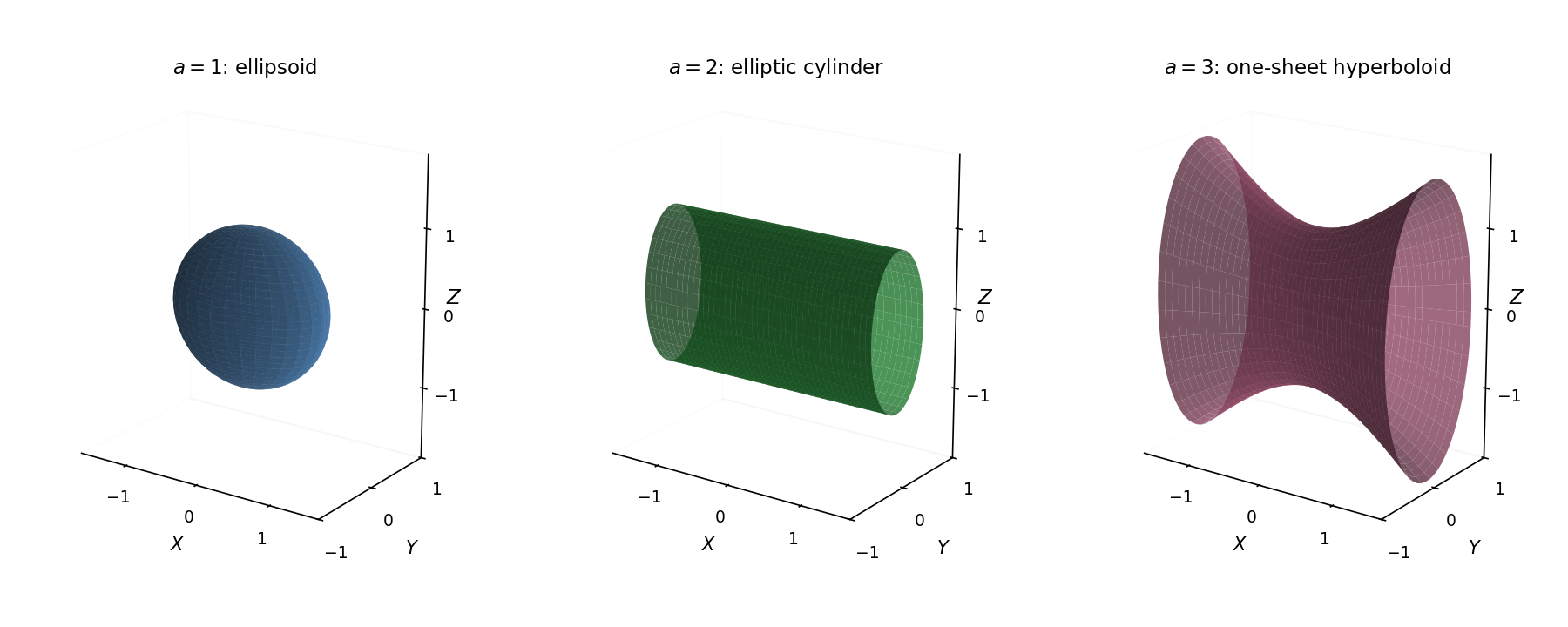
The block has characteristic polynomial . A convenient orthonormal eigenbasis for the full real symmetric matrix iswith eigenvalues , , and , respectively. Hence its orthogonal diagonalization isFor repeated eigenvalues, every nonzero combination within the corresponding eigenspace is also an eigenvector; the displayed basis remains valid. Introduce principal axes coordinatesThe quadratic form becomesThe principal-axis reduction of a quadric therefore has three regimes.
For , all coefficients are positive: the surface is an ellipsoid centred at the origin, withFor , the term disappears. The surface is an elliptic cylinder, unbounded along , whose cross-section is :For , there is one negative coefficient, so the surface is a one-sheet hyperboloid:Its waist at is an ellipse with semiaxes and . At other , both waist radii are multiplied by . There is no intercept on its longitudinal axis. Its asymptotic cone is . If positive eigenvalues coincide, the corresponding choice of principal axes is not unique, reflecting a rotational symmetry of the surface.

Using , the conjugate transpose of the proposed matrix isThusThe commutator of two Hermitian matrices is skew-Hermitian, and multiplication by changes it into a Hermitian matrix. No simplicity assumption on the spectra is needed for this part.
Suppose first that , and take an eigenvector of , with . Commutation givesSince the eigenvalue is simple, its eigenspace is one-dimensional, so for some scalar . Thus every vector in an eigenbasis of is also an eigenvector of . The simple spectrum of ensures these account for its eigenvector directions as well. Eigenvectors are understood up to nonzero scaling and permutation, rather than as literally identical numerical vectors.
Conversely, if are a common eigenbasis with and , thenfor every basis vector. Hence . ThereforeThis is simple spectrum gives simultaneous diagonalization. Without simple spectra, commuting Hermitian matrices still possess a common orthonormal eigenbasis, but not every arbitrary eigenvector of one matrix must be an eigenvector of the other.
Choose the common orthonormal eigenbasis established in part (ii), and let be the unitary matrix of its columns. ThenConsequentlyThus is unitarily diagonalizable, even though it need not be Hermitian. As a consistency check, commutation also gives , so is a normal matrix, as also follows from unitary diagonalization of a normal matrix.
Since is unitary, . Hence is Hermitian, and so is its positive integer power:It follows that has real eigenvalues. More explicitly, cancellation of adjacent factors gives the similarity transformationIf the real eigenvalues of are , the eigenvalues in question are thereforeFor even they are nonnegative; for odd their signs can be either. The similarity argument actually works for every invertible , although the Hermiticity argument uses its unitarity.
The Cauchy-Riemann equations give and . ThereforeTaking the nonnegative square root yieldsThe two gradients are also orthogonal, since , although equality of their lengths alone is the requested result.
Differentiate the prescribed imaginary part with respect to :The Cauchy-Riemann equation integrates toIts derivative is . On the other hand, . The second Cauchy-Riemann equation therefore requires . Combining the real and imaginary parts,Thus the most general answer on a connected domain isA real constant preserves the given imaginary part. Conversely, the difference of any two such analytic functions has zero imaginary part, and its Cauchy-Riemann derivatives force it to be constant. This proves completeness, rather than only exhibiting one possible harmonic conjugate.
For coefficients , the Cauchy-Hadamard theorem gives . HereThereforeOmitting the first two powers has no effect on the radius of convergence.
Let . For every fixed real , the base is positive once is sufficiently large; any initial negative or zero bases affect only finitely many coefficients. For that tail,The Cauchy-Hadamard theorem therefore yieldsFor example recovers the geometric-series radius one. The stronger expansion also shows that, on , the magnitudes of the individual terms tend to . Thus this series diverges at every point on its convergence circle; the radius itself does not require that extra boundary analysis.
The origin is an ordinary point of the Hermite differential equation, so put . Substitution and matching powers givesThus the linear recurrence relation isEven and odd coefficients evolve independently from arbitrary . The general power series solution iswith an empty product equal to one. Its first terms areBoth series converge at every finite , since the ratio of successive terms in each parity subsequence tends to zero. For a nonzero polynomial of degree , the highest coefficient in the differential equation requires . Conversely, at such a value the appropriate parity series terminates, while its opposite-parity initial coefficient can be set to zero. HenceHere is a physicists' Hermite polynomial. Two explicit choices areDirect differentiation verifies both. These are polynomial solutions up to an arbitrary overall factor. Without a polynomial requirement or additional boundary conditions, the equation also has nonpolynomial solutions for other real ; discreteness here comes from termination.
Insert the Frobenius solution and its differentiated series into the equation. Collecting the terms before shifting an index givesThe coefficient of the lowest power is . Because , the indicial equation givesFor the coefficient of with , shift the index in the second sum. The hypergeometric Frobenius recurrence isWhenever the left coefficient is nonzero, division yieldsFor noninteger , the two independent local solutions can therefore be identified aswith a consistent local branch for the fractional power. The hypergeometric function coefficients follow by iterating the recurrence using rising factorials.
There is a parameter qualification to the PDF's statement for all real constants: a zero denominator cannot be divided through. At an undetermined coefficient at Frobenius resonance, use the undivided coefficient equation to test compatibility. For example, requires , so a pure exponent-zero series with is impossible if . When the two indicial roots coincide, and a second independent solution generally needs a logarithmic term. The indicial roots and undivided relation remain the valid coefficient conclusions in these exceptional cases.
Define . For a density without explicit dependence, the chain rule givesThus the Euler-Lagrange equation implies the Beltrami identityWhere this first integral is equivalent to the original equation. At a turning point it extends by continuity. On an entire constant segment, however, its derivative alone can vanish without imposing the full Euler-Lagrange equation, so such candidate paths must still be checked in the original equation.
The monotonic horizontal coordinate allows the path to be written as a graph. Its arc length element is , so the variational density is . It has no explicit horizontal-coordinate dependence. The Beltrami identity becomesConsequently every smooth minimizing path satisfiesThis is a first integral of the weighted arc-length problem; fixed endpoint values remove the endpoint variation terms.
Interpret the density on the physical region . It is singular at zero and would not describe a nonnegative density for . The first integral gives for a positive constant . To handle the horizontal tangent without dividing by , use the full Euler-Lagrange equation:Two integrations give . The equal endpoint heights force , and either endpoint then gives . ThusThe path is the upper circular arc. A constant horizontal path solves the differentiated first integral trivially but fails , so is not another extremum.
One can prove global minimality, rather than only stationarity. Define on the upper half-plane. ThenThe Cauchy-Schwarz inequality gives, along any admissible path from to ,Our circle has tangent for increasing , so equality holds pointwise. This calibration for semicircular hyperbolic geodesics provesThe geometry is that of a hyperbolic geodesic in the Poincaré half-plane model. The proof even allows competing upper-half-plane paths beyond the class of monotonic graphs.
The path rises from to its maximum height at , then falls symmetrically to . Its radius is , and its endpoint polar angles are and , giving angular span . Hence its ordinary arc length isEquivalently, and integrating over gives the same value. This Euclidean length differs from the weighted destruction integral : the slightly longer route saves undergrowth by travelling at greater height.
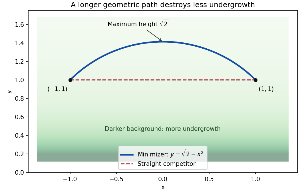
The least-destruction path bends towards lower density
. Original exact semicircular minimizer and its horizontal competitor. The shaded background indicates the density in the upper half-plane. The minimizer has Euclidean length but weighted cost , smaller than the straight path's cost two. Details.
Self-adjoint form. Grouping the two derivative terms gives . Thus a regular Sturm-Liouville operator isThe boundary conditions are mixed Neumann boundary conditions at zero and Dirichlet boundary conditions at . For , , and , as required. The boundary term vanishes for two functions satisfying these conditions, confirming self-adjointness on that domain.
Constrained variation. Introduce a Lagrange multiplier for the normalization and varyIts first variation isThe endpoint term vanishes because and . The Euler-Lagrange equation is thereforewhich is exactly the original eigenvalue problem for the boxed choices of . Multiply by and integrate by parts. The same endpoint conditions giveThus the stationary functional values are the eigenvalues, with . More generally, before normalization the relevant Rayleigh quotient is
Unperturbed ground mode. At , the equation is . The quadratic form is nonnegative, and zero eigenvalue would force a constant function incompatible with the endpoint at . For positive , . The derivative condition forces , while the other endpoint gives . HenceThe lowest eigenvalue and normalized eigenfunction are
Trial-function bound. The Rayleigh-Ritz method says that the minimum eigenvalue is no larger than the quotient of any admissible trial function. The same still satisfies both boundary conditions and retains unit norm. Its derivative is , givingUsing ,Therefore the affine-parameter Sturm-Liouville eigenvalue bound isThis is an upper bound for every , not merely a small-parameter approximation. As a lower-bound check, and the unperturbed variational minimum imply for every admissible normalized . Thus
Articles by others on the same topic
There are currently no matching articles.