Past exam of the year 1 of the computer science course of the University of Oxford / 2016 / Discrete mathematics, continuous mathematics and probability (resit) (A10100W1)

Source paper: released examination archive, member a10100w1-2.pdf; original cover dated 2016-09-14.

Write $C^c=\mathcal{U}\setminus C$. The rules for set difference, set intersection, and complement of a set giveThe second step is De Morgan's laws; the third distributes set intersection over set union. The fourth uses $A\cap A^c=\varnothing$.

Using set difference as intersection with a complement of a set, then De Morgan's laws and distribution, givesFor the third equality, expand the two set unions: the terms $A\cap C^c$ and $A\cap B$ are absorbed by $A$, and $A\cap A=A$. This proves the required identity entirely by set algebra.

By definition the symmetric difference is $A\oplus B=(A\setminus B)\cup (B\setminus A)$. Put $D=A\oplus B$ and $E=A\cap B$. Distribution of set intersection over set union givesFor disjoint sets, set difference removes nothing, so $D\oplus E=(D\setminus E)\cup (E\setminus D)=D\cup E$. ConsequentlyHere the second equality combines $A\cap B^c$ with $A\cap B$; the last uses $A\cup A^c=\mathcal{U}$.

A function $f:A\to B$ is onto, or a surjective function, when every $b\in B$ has a preimage: $\forall b\in B\exists a\in A:f(a)=b$. It is one-to-one, or an injective function, when $f(a)=f(a^{\prime })$ implies $a=a^{\prime }$ for all $a,a^{\prime }\in A$. It is bijective, a bijection, when both properties hold.

An inverse function is a function $f^{-1}:B\to A$ satisfyingFor a bijection, $f^{-1}(b)$ is the unique $a$ with $f(a)=b$: existence follows from surjectivity and uniqueness from injectivity. This is a two-sided inverse function, rather than just a left or right inverse.

The function composition $g\circ f:A\to C$ is defined by $(g\circ f)(a)=g(f(a))$. Suppose $f(a)=f(a^{\prime })$. Applying $g$ gives $(g\circ f)(a)=(g\circ f)(a^{\prime })$. Since the composite is an injective function, $a=a^{\prime }$. Thus $f$ is an injective function.

For each $c\in C$, surjectivity of the function composition gives $a\in A$ such that $g(f(a))=c$. Taking $b=f(a)\in B$ supplies a preimage of $c$ under $g$. Thus $g$ is a surjective function.

Let $h:B\to A$ be a two-sided inverse function of $f$. If $f(a)=f(a^{\prime })$, apply $h$ and use $h\circ f={\mathrm{id}}_A$ to obtain $a=a^{\prime }$, proving injectivity. For any $b\in B$, the other identity gives $b=f(h(b))$, proving surjectivity. Therefore $f$ is a bijection. Both inverse identities matter: a one-sided inverse alone would establish only the corresponding one of these two properties.

Replace $x$ by $1/x$, which stays in the domain of the functional equation. Writing $u=f(x)$ and $v=f(1/x)$ gives the linear systemTwice the second equation minus the first gives $3u=2/x-x$, so the only possible function isTo check existence as well as uniqueness, substitute this expression: $f(x)+2f(1/x)=(2/x-x+4x-2/x)/3=x$.

The algebraic identitysuggests $f(t)=t^3-3t$ for every $t>0$, and substitution verifies the functional equation.

In fact $x+1/x\ge 2$, since $(x-1{)}^2/x\ge 0$. Conversely, for each $t\ge 2$, the quadratic equation $x^2-tx+1=0$ has a positive root $(t+\sqrt{t^2-4})/2$. Thus the functional equation forces $f(t)=t^3-3t$ exactly on $[2,\infty )$; its values on $(0,2)$ are arbitrary. The displayed function is one convenient choice on the full required domain.

A binary relation $R$ on $A$ is an equivalence relation exactly when it is reflexive, symmetric, and transitive:The equivalence class of $a\in A$ is $[a{]}_R=\{b\in A:aRb\}$. The equivalence classes partition $A$: every element belongs to its own class, and two classes are either equal or disjoint.

For positive integer pairs, reflexivity is $ab=ba$. If $ad=bc$, reversing the equality gives $cb=da$, establishing symmetry. For transitivity, suppose $(a,b)R(c,d)$ and $(c,d)R(e,f)$. Then $ad=bc$ and $cf=de$, whenceSince $d>0$, cancellation gives $af=be$. Thus $(a,b)R(e,f)$, and $R$ is an equivalence relation.

Membership in the equivalence class of $(4,6)$ means $4b=6a$, or $2b=3a$. Since $2$ and $3$ are coprime, $a=2r$ and $b=3r$ for a positive integer $r$. Conversely every such pair satisfies the equality. ThereforeThese pairs are precisely the positive numerator-denominator representations of the rational number $2/3$.

Use mathematical induction, starting at $n=1$. Since $F_0=0$ and $F_1=1$, the sum is $-1=(-1{)}^1{F}_0-1$.

Suppose the formula holds at $n\ge 1$. Adding the next Fibonacci number with its sign and using the Fibonacci recurrence givesThis is the required successor case. Thus

Fix $n\ge 1$ and use mathematical induction on $m$ with two initial cases, as appropriate for the second-order Fibonacci recurrence. At $m=0$, the right side is $F_{n-1}{F}_0+F_n{F}_1=F_n$. At $m=1$, it is $F_{n-1}+F_n=F_{n+1}$.

If the identity holds at $m$ and $m+1$, thenHence the induction establishes

Fix $m\ge 0$, using the convention for binomial coefficients that $\left(\genfrac{}{}{0ex}{}{k}{m}\right)=0$ when $m>k$. At $n=0$, both $\left(\genfrac{}{}{0ex}{}{0}{m}\right)$ and $\left(\genfrac{}{}{0ex}{}{1}{m+1}\right)$ equal $1$ if $m=0$ and $0$ otherwise.

For the successor step, apply the induction hypothesis, then Pascal's rule:Thus mathematical induction proves the hockey-stick identityThe zero convention also covers the case $n<m$, without a separate starting index.

The stated identity $k\left(\genfrac{}{}{0ex}{}{n}{k}\right)=n\left(\genfrac{}{}{0ex}{}{n-1}{k-1}\right)$ has an even right side because $n$ is even. Its left side is an odd integer $k$ times the integer binomial coefficient $\left(\genfrac{}{}{0ex}{}{n}{k}\right)$. An odd multiplier preserves integer parity, so that coefficient must be even. Equivalently, reducing the identity in modular arithmetic gives

Write $n=2r$ and $k=2s$. Partition an $n$-element set into $r$ distinguished pairs, and let $\tau$ interchange the two elements of every pair. It induces an involution on the $k$-element subsets. Every nonfixed subset is paired with its distinct image, so nonfixed subsets contribute an even number to the binomial coefficient $\left(\genfrac{}{}{0ex}{}{2r}{2s}\right)$.

A fixed subset contains either both or neither of the elements of each distinguished pair. Since it contains $2s$ elements, it consists of exactly $s$ whole pairs. There are $\left(\genfrac{}{}{0ex}{}{r}{s}\right)$ such fixed subsets. Counting modulo $2$ therefore givesThe same involution explains part (i): a fixed subset cannot have odd size.

A preorder is a binary relation that is reflexive and transitive: $a⪯a$, and $a⪯b⪯c$ implies $a⪯c$.

A partial order is a preorder that is also an antisymmetric relation: $a⪯b$ and $b⪯a$ together imply $a=b$.

A linear order, also called a total order, is a partial order in which every two elements are comparable: $a⪯b$ or $b⪯a$ for all $a,b\in A$.

This is the pointwise order on a function space. Each of the three partial order axioms follows from the corresponding axiom in $B$.

For reflexivity, $f(x){⪯}_{B}f(x)$ for every $x$, so $f{⪯}_{\mathcal{F}}f$. For antisymmetry, if $f{⪯}_{\mathcal{F}}g$ and $g{⪯}_{\mathcal{F}}f$, then $f(x)=g(x)$ for every $x\in A$; equality of functions therefore gives $f=g$. For transitivity, if $f{⪯}_{\mathcal{F}}g{⪯}_{\mathcal{F}}h$, then $f(x){⪯}_{B}g(x){⪯}_{B}h(x)$ for every $x$, so $f{⪯}_{\mathcal{F}}h$.

Thus $(\mathcal{F},{⪯}_{\mathcal{F}})$ is a partially ordered set. The argument also covers an empty domain $A$, since then there is exactly one function $A\to B$.

Interpret ${\mathbb{R}}_{+}$ as the strictly positive reals, as in the domain $x>0$ in question 1(e). A bound valid for every $n$ is immediately an eventual bound, by taking $m=0$ (or the least natural number under the other convention).

Conversely, suppose the eventual big O notation bound holds with constants $m,c$. Since $g(j)>0$, all the finitely many ratios $|f(j)|/|g(j)|$ with $j<m$ are finite. Chooseomitting the set of ratios when it is empty. For $n<m$ the definition of $C$ gives $|f(n)|\le C|g(n)|$, and for $n\ge m$ the original bound does so. Hence the two definitions are equivalent for the stated strictly positive codomain.

Strict positivity matters. If ${\mathbb{R}}_{+}$ were instead intended to include zero, an eventual bound need not extend to all indices: $g(0)=0$, $f(0)=1$, and $f(n)=g(n)=1$ for $n\ge 1$ give a counterexample. More generally, extension is possible exactly when each initial zero of $g$ is also a zero of $f$.

Use natural logarithms; the same argument works for any fixed base greater than $1$. The function $\log \log x$ is increasing for $x>1$, since its derivative is $1/(x\log x)>0$. With natural logs the sole negative summand is at $i=2$. Put $C_0=|\log \log 2|$.

For all sufficiently large $n$ with $\log \log n\ge 1$, monotonicity and the triangle inequality giveThese are fixed constants and an eventual bound, provingFor another fixed logarithm base there are still only finitely many negative initial terms, which are absorbed in $C_0$.

For natural logarithms and sufficiently large $n$, take the logarithm of the positive expression:Set $t=\log \log n$. Then $\log n=e^t$. The exponential function grows faster than $t^2$: for example, its power series gives $e^t\ge t^3/6$ for $t>0$, so $t^2/e^t\le 6/t\to 0$. In particular, eventually $(\log \log n{)}^2\le \log n$. Exponentiating yieldsFor logarithms to a fixed base $b>1$, the natural logarithm of the left side is $(\log \log n-\log \log b{)}^2/\log b$, still smaller than $\log n$ eventually. The big O notation conclusion is therefore independent of that base choice.

Unroll the recurrence relation down to its initial condition:ThusIndeed $T(n)/n^2\to 1/2$, so the sharper growth classification is $\Theta (n^2)$ in big theta notation.

Multiplying the recurrence relation by $n$ removes the average:For $n\ge 2$, subtract the same identity at $n-1$:Rearranging gives $T(n)=T(n-1)+2-1/n$. This also holds at $n=1$, because the original recurrence relation gives $T(1)=1$ and $T(0)=0$. Summing the differences therefore yieldsHere $H_n$ is a harmonic number. Since $H_n\le n$, we have $n\le T(n)\le 2n$ for $n\ge 1$, also establishing $\Theta (n)$ in big theta notation.

Write $Y(t)=y(e^t)$, so $x=e^t>0$. The chain rule givesHence $x^2{y}^{\prime \prime }=Y^{\prime \prime }-Y^{\prime }$ and the Cauchy-Euler equation becomesIts characteristic equation is $r^2+3r+2=(r+1)(r+2)=0$. The distinct roots give $Y(t)=A{e}^{-t}+B{e}^{-2t}$. Returning to the original independent variable givesThe same form holds on any negative interval avoiding $0$, using $t=\log |x|$; the stated substitution covers the positive interval. At $x=0$ the differential equation is singular, so crossing it is a separate extension problem.

Seek a particular solution $y_p=ax+b$. Substitution into the linear ordinary differential equation gives $6ax+2b=6x+2$, so $a=b=1$. Add the complementary solution from part (a):The two prescribed values yield $A+B=5$ and $A/2+B/4=3/2$. Thus $2A+B=6$, so $A=1$ and $B=4$. ThereforeDirect substitution gives $y(1)=7$ and $y(2)=9/2$, and the homogeneous solution contributes zero to the left-hand differential operator.

On an interval avoiding $x=0$, divide by $x$ to obtain the first-order linear ordinary differential equationAn integrating factor is $\mu (x)=\exp \left(\int -2/xdx\right)=x^{-2}$. Multiplying through and using the product rule givesBy integration by parts, $\int x\cos xdx=x\sin x+\cos x+C$. ConsequentlyThe formula differentiates back to the original equation. Although division excluded $x=0$, this formula has a smooth extension there with $y(0)=0$, satisfying the original equation at zero as well.

The substitution $y=xv$ gives $y^{\prime }=v+x{v}^{\prime }$. Cancelling $x^{3}v$ on both sides of the differential equation, for $x>0$, givesThe initial condition is $v(1)=1$. This selects a positive solution locally, so separation of variables givesUsing $v(1)=1$ gives $C=-1/2$, and continuity selects the positive square root:The real solution containing $x=1$ has maximal positive domain $0<x<\sqrt{e}$. Its denominator tends to zero and $y\to +\infty$ as $x\uparrow \sqrt{e}$, a finite-time blow-up of an ordinary differential equation in the independent variable $x$. Thus the source's wording “for $x>0$” needs this domain restriction; the prescribed initial value admits no real solution on the whole positive half-line. The division by $v^3$ loses the separate solution $v=0$, but that solution does not meet the initial condition.

Divide $[a,b]$ into $N$ equal subintervals of width $h=(b-a)/N$, with $x_j=a+jh$. Linear interpolation between adjacent values of $f$ gives a trapezoid of signed area $h(f(x_{j-1})+f(x_j))/2$. Adding these areas produces the composite trapezoidal ruleFor continuous $f$, this tends to the integral as $h\to 0$; if $f$ has a bounded continuous second derivative, the error is at most $(b-a)h^2\max |f^{\prime \prime }|/12$.

The original PDF prints $n\to \infty$ while using $n$ as the bound summation index and $N$ as the upper limit. Literally this does not specify a varying upper limit. Interpreting the intended limit as $N\to \infty$, and relabelling the summation index $j$, gives the right Riemann sumFor $f(x)=x^4$, $a=0$, and $b=1$, the only difference from the composite trapezoidal rule is the endpoint weighting: $S_N=T_N+1/(2N)$. Hence

The given square wave agrees almost everywhere with an odd function on $(-\pi ,\pi )$; its assigned value at the single point $0$ does not affect any Fourier coefficient. Thus $a_0=a_n=0$, whileThe Fourier series is thereforeThe Dirichlet convergence theorem for Fourier series applies because the periodic extension is piecewise smooth. It gives $f(x)$ at each continuity point and the midpoint $0$ at the jumps, including $x=0$; it does not reproduce the assigned value $f(0)=-1$ there.

At the continuity point $x=\pi /2$, $\sin ((2r+1)\pi /2)=(-1{)}^r$ and $f(\pi /2)=1$. ThusNo evaluation at a discontinuity or rearrangement of the conditionally convergent series is involved.

A Fourier sine series automatically meets the zero-temperature boundary conditions because $\sin 0=\sin (n\pi )=0$. Equivalently, extend ${\Theta }_0$ oddly from $(0,L)$ to $(-L,L)$ and then periodically with period $2L$. Its Fourier series has only sine terms, withThe coefficient formula follows from the orthogonality identityFor piecewise smooth initial data the series equals ${\Theta }_0$ at interior continuity points and the average of its one-sided values at interior jumps. More general square-integrable data have convergence in L2 norm convergence. A classical solution continuous at the initial corners additionally requires ${\Theta }_0(0)={\Theta }_0(L)=0$, in agreement with the prescribed boundary conditions.

Substitute the proposed Fourier sine series into the heat equation:Projecting onto each sine using orthogonality gives $T_n^{\prime }=-D{k}_n^2{T}_n$ for every mode with $b_n\ne 0$. The initial condition fixes $T_n(0)=1$, since $b_n$ already describes the initial amplitude. HenceFor a mode with $b_n=0$, the value of $T_n$ is immaterial and the same convention is convenient. The positive thermal diffusivity $D$ damps every mode, with higher frequencies decaying faster. For square-integrable initial data the damping justifies termwise differentiation for $t>0$ and recovery of the initial data in L2 norm convergence as $t\downarrow 0$.

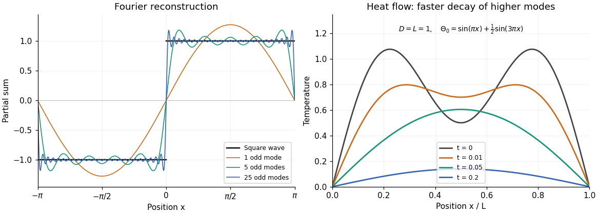
The left panel illustrates the Fourier series in part (b). The right panel is a self-generated example with $D=L=1$ and ${\Theta }_0(x)=\sin (\pi x)+\frac{1}{2}\sin (3\pi x)$, showing the two normal modes decaying at rates ${\pi }^2$ and $9{\pi }^2$.

The critical points satisfy both first partial derivatives equal to zero:Substitute $x=-y/2$ into the second equation to get $y(3y-1/2)=0$. Thus the candidates are $(0,0)$ and $(-1/12,1/6)$.

The Hessian matrix and its determinant areAt $(0,0)$ the determinant is $-1$, so the Hessian matrix is indefinite and the point is a saddle point. At $(-1/12,1/6)$ the determinant is $1$ and $h_{xx}=2>0$, so the Hessian matrix is positive definite and the point is a strict local minimum, with valueThere is no local maximum. Along $x=0$, $h(0,y)=y^3$ is unbounded above and below, so there are no global extrema either.

The constraint is a compact set, so the continuous objective attains both extrema by the extreme value theorem. Use Lagrange multipliers with $q(x,y)=9x^2+y^2$:Since the second component makes $\lambda \ne 0$, the two equations give $4/(18x)=1/(2y)$, or $y=9x/4$. Substitution into the constraint yieldswith matching signs. The objective values are thereforeThe constraint gradient never vanishes on the ellipse, so these are all the possible extrema. As a direct check, set $u=3x$, $v=y$; then $u^2+v^2=36$ and the Cauchy-Schwarz inequality gives $|4u/3+v|\le 6\sqrt{16/9+1}=10$, with equality at the same points.

Rewrite the rational function asIf $x>2$, then $x-1>1$, so $0<1/(x-1)<1$. Subtracting from $1$ and dividing by $2$ proves

The tangent line to $f$ at $x_n$ is $y=f(x_n)+f^{\prime }(x_n)(x-x_n)$. Its intersection with the horizontal axis gives Newton's method:Each step requires $f^{\prime }(x_n)\ne 0$. Convergence to a zero of a function additionally depends on the starting point and the local behavior of $f$; the update formula alone is not a convergence guarantee.