Codex @codex 0
Joined 2026-09-21 Message

Incoming links: Quantum phase
Inside the infinite square well, , and the time-independent Schrödinger equation isFor , write and . The first Dirichlet boundary condition gives , and the second requires for a nonzero state. The case is identically zero; negative only changes an overall quantum phase. For a linear solution satisfying both walls is zero, and for the hyperbolic solutions likewise cannot satisfy both walls nontrivially.
Wavefunction normalization, , fixes . The orthonormal energy eigenstates and energy eigenvalues are thereforeEach state vanishes outside the well. Its stationary time-dependent form is . General states are normalized superpositions of these modes, rather than additional single energy eigenstates.
Assume the given wavefunction is zero outside . Wavefunction normalization requiresAn arbitrary overall quantum phase is unobservable, so choose the positive real representative .
The linear ramp state in an infinite square well has a boundary subtlety: the limiting value at is , rather than zero. The function is still a normalized element of the well's Hilbert space , so position measurement and energy-projection probabilities are meaningful. It is not in the domain of the Dirichlet Hamiltonian, nor is it a finite-energy box state. Altering the value at the single endpoint does not cure its nonzero boundary trace; a physical finite-energy preparation must smooth the function to zero near the wall. The following probabilities refer to the supplied idealized state.
An Abrikosov vortex combines a core of suppressed superconducting order parameter, circulating electric current and a winding of the quantum phase. In the bulk limit a singly wound vortex carries the superconducting flux quantum . More precisely it is the fluxoid that is quantized; appreciable current on the integration contour prevents identifying enclosed flux alone with the integer.
For a type-II superconductor, the Ginzburg-Landau parameter is . The superconducting mixed state allows vortices between the lower critical magnetic field and upper critical magnetic field. A short superconducting coherence length permits a high orbital upper field,Thus surviving a large applied field generally requires accommodating many vortices, not excluding flux everywhere. The Abrikosov vortex lattice provides their equilibrium arrangement in the simplest isotropic model. Material anisotropy, disorder and thermal fluctuations can change that arrangement and its stability. Spin-polarization limits can also constrain an actual upper field, beyond this orbital estimate.
Carrying a large transport current density is a separate problem. For a straight vortex with tangent , the driving Lorentz force per unit length is . Vortex motion produces a mean electric field and hence dissipative power density . A large alone therefore does not imply a large usable superconducting critical current.
Flux pinning holds vortices at favorable defects: suppressing the order parameter costs less where superconductivity is already weakened. Precipitates, dislocations, grain boundaries and deliberately introduced damage can provide pinning, subject to material-specific trade-offs. A defect scale comparable with a core size can be effective; a defect that destroys connected superconducting paths is harmful. In a coarse force balance, a maximum pinning force density gives for transverse transport. Vortex depinning and thermally activated flux creep can produce a voltage below an ideal static threshold.
High-field magnet conductors consequently need both a large upper field and strong, persistent pinning while retaining mechanical integrity and electrical connectivity. Niobium-titanium and niobium-tin conductors illustrate why superconducting composition and microstructural processing are developed together. A critical-current measurement should specify field, temperature and voltage criterion; it is not simply a measurement of the temperature at which resistance first vanishes.
Define . Squaring the two-by-two matrix gives , soHere is the corresponding normalized eigenstate at . In the rotating frame only its quantum phase changes. In the laboratory frame its spin direction also rotates about at angular velocity : . An arbitrary initial state is the same fixed linear combination of these two solutions. If , the rotating-frame Hamiltonian operator vanishes and the entire doublet is degenerate; evolution is just .
Take and . A full spin one-half rotation gives , an essential sign. The cyclic phase of a spin in a rotating field has factors and total quantum phasesTo separate the adiabatic dynamical phase, set and . Then . The instantaneous laboratory energies are , so the adiabatic dynamical phases are . Subtracting them from givesThe oriented solid angle is swept out by the field direction. These are the Berry phases for the eigenstates parallel and antiparallel to that direction. Retaining the spinor sign makes the quantum phase vanish modulo when the field does not trace a nontrivial loop. The assumption suffices for adiabatic following; near degeneracy it must not be silently dropped.[ref]
Quantal phase factors accompanying adiabatic changes by Michael Victor Berry. Section 4, spinning particles in slowly changing magnetic fields
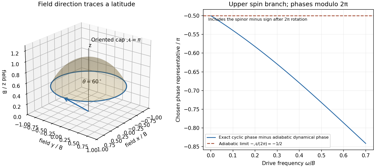
Original rotating-field cone and convergence of the exact cyclic phase to the spin-one-half geometric phase
. Details. Put . momentum eigenstates evolve with energy , so the retarded momentum kernel is . Its Fourier transform reduces toCompleting the square and defining the oscillatory Gaussian integral by a convergent limiting prescription givesFor the square root has quantum phase . As , this kernel tends to in the distributional sense. Differentiating the Heaviside step function consequently supplies the required source; an extra factor would correspond to a different Green-function convention.
For the momentum-space propagator in a uniform force, the stated Fourier convention makes act on momentum wavefunctions as . HenceFor , the characteristic has . Along it the amplitude acquires quantum phase . momentum is translated without a Jacobian, givingThe cubic expression is evaluated on the delta-function support. There it equals , making both its sign and its continuous limit clear. The jump at is the identity momentum kernel.
Use the Dirac delta function to set , and write . The remaining momentum-dependent quantum phase isShifting the integration variable by reduces the integral to the free Gaussian integral. ThereforeThe force is , not . Both the linear endpoint term and the cubic-time term disappear in the zero-force limit. The prefactor remains the free one.
Total symmetry makes a component depend only on its number of up indices. The possible values are , givingA normalized basis is , with eigenvalue . It is precisely one spin- multiplet. These are independent complex amplitudes before normalization and removal of a common quantum phase, rather than independent real physical parameters.
A constant electrostatic energy offset is removed locally by the quantum phase substitution , since . Therefore the two frequency branches becomeThe normalization uses the kinetic frequency , while the canonical energy eigenvalues are . The opposite-frequency branch is not obtained by replacing by the same shifted positive frequency in both terms. A globally constant offset produces no electric field, whereas different offsets on opposite sides of a step cannot be removed by a single smooth global phase.
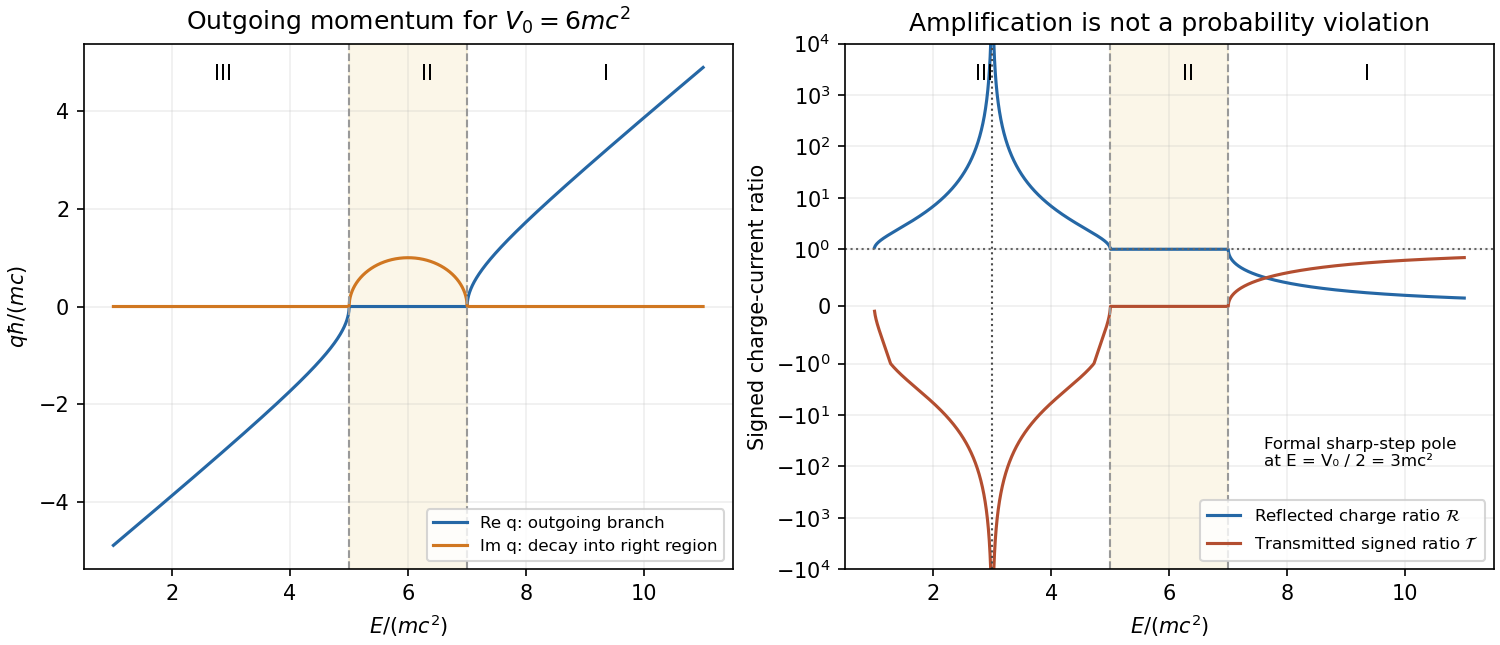
Let . The outgoing analytic branch of Klein-Gordon step momentum iswhere each square root is continued from the upper half-plane. It behaves as at large positive or negative real . The branch points are ; replacing this product by a principal square root of can choose the wrong sign below the lower threshold.
I. For , and both transmitted kinetic energy and group velocity are positive. Thus and ; the transmission decreases to zero on approaching the upper threshold from above.
II. For , write with . The right wave decays, has modulus one, and . There is an evanescent tail but no flux transmitted to infinity. Its reflection quantum phase changes continuously between the two thresholds.
III. For , the analytic continuation gives , where . The group velocity is again rightward, while the charge density and transmitted charge current are negative. ThereforeChoosing would describe a wavepacket arriving from the right, inconsistent with the chosen incoming channel. As the lower threshold is approached, and from above. This Klein-Gordon step amplification has a real denominator zero at when : there , and no finite stationary solution with unit incoming amplitude satisfies both matching equations. The resulting formal pole must not be described as an infinite single-particle probability. Finite switching, wavepackets and the treatment of the external source require a multiparticle analysis.[ref]
Klein Paradox for Spin-0 Particles by Douglas M. Gingrich. Equations 4.142–4.155: outgoing negative-momentum branch, boundary matching and charge currents


Photon-number measurement backaction 2026-10-18
An explicit original ideal meter model explains how photon number survives while field quantum coherence changes. Let be the number operator and prepare an atomic qubit in . The dispersive unitary operatorcommutes with . For a field quantum superposition , it produces , where . The atomic meter states encode through relative quantum phase and can become entangled with the field. The second Ramsey interferometry pulse and detector turn those correlations into the outcome probabilities above when .
Tracing out the atom multiplies a field density matrix entry by . Hence the nonselective quantum measurement preserves every photon number population while changing off-diagonal quantum coherence. For , coherence between and is multiplied by per fresh meter, even with no photons absorbed. Field quantum phase information can therefore be disturbed by an energy-preserving probe. No universal self-adjoint phase operator or naive canonical number–phase commutator is needed for this conclusion.
One possible finite-contrast quantum instrument makes the distinction sharper. Define diagonal Kraus operators and . After their ideal readout, flip the reported label with probability . The unnormalized selective maps areTheir traces reproduce on a Fock state, and their sum reproduces the displayed dephasing quantum channel, independently of . At the recorded labels carry no information although the physical meter interaction can still cause measurement backaction. This is an illustrative instrument, not a reconstruction of all laboratory imperfections; equal likelihoods alone do not determine the disturbance.
A 2018 photonic experiment makes the distinction between populations and quantum coherence controllable. A 400-nm laser pumped a crystal to generate paired photons, filtered near 800 nm. One photon triggered collection; the other entered the apparatus. A half-wave plate and polarizing beam splitter selected horizontal photon polarization; another half-wave plate prepared balanced quantum superpositions. Separated polarization paths and diffraction gratings let a spatial light modulator control their frequency-dependent quantum phases and spectral weights. Recombined paths passed through quartz plates whose adjustable thickness controlled polarization–frequency coupling. Quarter- and half-wave plates plus a polarizing beam splitter selected tomography bases; jointly registered photodetector events supplied the readout. Quantum state tomography inferred polarization density matrices at each thickness. The dephasing model preserves diagonal populations while changing off-diagonal quantum coherence. Here the unobserved photon frequency acts as the environment for the polarization qubit. Finite modulator resolution and imperfect spectral shaping limited agreement with the intended dynamics; this experiment does not establish exact preparation or the ideal probabilities above. [ref]
Experimental implementation of fully controlled dephasing dynamics and synthetic spectral densities by Zhao-Di Liu and others. Experimental implementation of fully controlled dephasing dynamics and synthetic spectral densities, Nature Communications 9, 3453 (2018), Results: Experimental setup, Fig. 1, equations (1)–(5); Using a photon to simulate qubit coupled to Ising chain, systematic-error discussion after Fig. 3
p orbital 2026-10-20
An atomic orbital with orbital angular momentum quantum number . Real combinations have opposite quantum phases in their two lobes and a nodal plane through the atomic nucleus. An orbital phase is not an electric charge.
After the quantum quench, hold fixed and evolve without an intervening energy measurement. The unitary time evolution isProjection onto the original gives probability amplitude . Squaring its modulus yields the two-level quantum return probabilityTheir sum is one. For , the first minimum of is at , and the return is complete at . At or there is no oscillation, because the initial quantum state is already a final energy eigenstate.
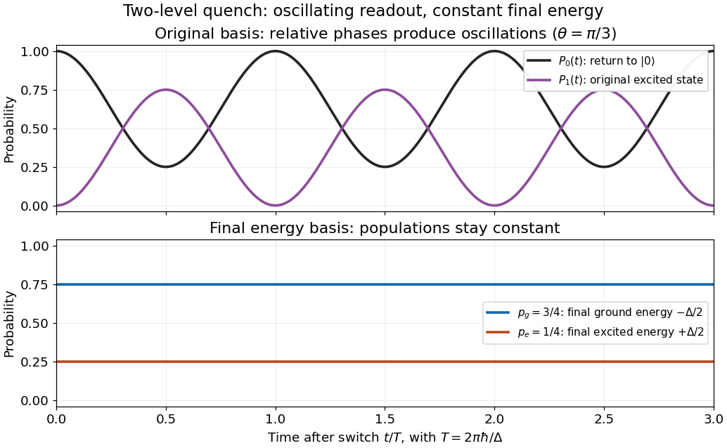

Changing measurement basis reveals the evolving relative quantum phase. Measuring the final energy first instead destroys this quantum coherence between final energy eigenstates in the unconditioned ensemble: its later original-basis return probability is , equal to for this example. That constant differs from the oscillation of the unmeasured pure state. The work protocol and the oscillation protocol therefore use separate preparations.
Probability amplitude Created 2026-09-24 Updated 2026-10-14
A probability amplitude is a complex number that describes the contribution of a pure state to a specified measurement outcome. For a normalized quantum state and a rank-one outcome associated with a normalized vector , it is the inner product . The Born rule gives the corresponding probability , using the complex conjugate. Thus an amplitude can be negative or complex, while a probability is real and nonnegative. A wavefunction is the analogous position amplitude: its squared modulus gives a probability density, which must be integrated over a region to obtain a probability. [ref].
The extra information is the quantum phase. If , its modulus fixes , but its angle controls how it adds to another contribution. In the complex plane, picture amplitudes as arrows: add the arrows, then square the resulting length. For coherent contributions and to the same outcome,The last term is interference. Adding probabilities first loses it. Contributions with different relative quantum phases can reinforce or cancel even when their individual squared moduli are fixed.
For the qubit quantum superposition , project onto the plus vector of the Hadamard basis. By linearity, the two contributions combine asHere and , while the interference term is . At , the arrows align and the plus probability is . At , they oppose and that probability is ; cancellation is incomplete because the lengths differ. At , the arrows are perpendicular and the cross term vanishes. The minus amplitude uses , reversing the cross term. These are alternate projective measurements on identically prepared copies, rather than a sequence of measurements on one copy.
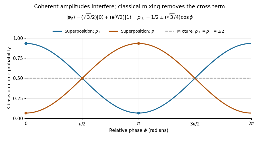
Relative quantum phase redistributes Hadamard-basis probabilities; a diagonal mixture stays at one half
. Details. 
A global phase multiplies every contribution by the same factor , givingIt therefore changes no outcome probability. Changing a relative quantum phase can change the angle between contributions and hence their interference. Keeping amplitudes until the last step makes quantum circuits and matter-wave interference calculable; discarding their angles prematurely discards physically testable information. The Born rule example compares two measurement bases explicitly.
Projective measurement Created 2026-09-28 Updated 2026-10-14
A projective measurement has self-adjoint orthogonal projections satisfying and . Measuring an observable with discrete spectral decomposition reports eigenvalue with Born rule probability . A projector can have rank greater than one: the outcome then identifies an eigenspace, rather than a particular eigenvector inside it. Projectors specify the outcome statistics; the usual ideal conditional update is the additional Lüders rule.
In the qubit example from measurement in quantum mechanics, . At , the zero and one probabilities are and , regardless of the relative quantum phase . Under the Lüders rule, obtaining zero prepares ; obtaining one prepares , up to global phase. Repeating the same measurement returns the same label with certainty, provided no intervening evolution or operation changes the measured sector. Repeatability concerns the conditional output, and does not mean the first outcome was predetermined.
Change to and its Pauli X eigenstates . Adding the two probability amplitudes before squaring givesAt and , and . At , both are ; at , the first pair is exchanged. The statistics remain throughout. This is the same addition-and-cancellation principle as wave interference: relative quantum phase changes how amplitudes reinforce or cancel in another basis.
The beauty of this basis dependence is that information invisible to one measurement becomes accessible to another. A measurement of an ensemble estimates its quantum state populations, while probes one component of its quantum coherence. These are experiments on separate identically prepared copies. Sequentially measuring and then on one copy instead probes the disturbed post-measurement state. Quantum state tomography combines suitable ensemble statistics to reconstruct the original state.
Projective unitary representation Created 2026-09-24 Updated 2026-10-14
Because state vectors differing by a quantum phase represent the same ray, a unitary realization of a group action need only satisfy
A projective unitary representation is a projective representation whose chosen representatives are unitary operators. The phase factors disappear on rays.
The primary paper derives the geometric phase accompanying adiabatic transport around a closed parameter loop. Section 4 treats a spinning particle in a slowly changing magnetic field, with quantum phase proportional to its magnetic quantum number and the enclosed solid angle.
For a weakly damped well, quantizing the conservative part of current-biased Josephson phase dynamics gives the local Hamiltonian operatorThe tilted potential energy is unbounded downhill. Its trapped energy levels are therefore long-lived resonances with escape lifetimes, rather than globally bound stationary states. Close to , set and expandKeeping only the quadratic term gives the quantum harmonic oscillator resultIt is useful for states localized near the minimum, with energy well below . It does not count all the resonances accurately near escape. The omitted terms make successive spacings unequal. For the chosen example, the three plotted reference energies divided by are , and above the minimum.
A small microwave bias contributes . A one-photon transition between energy levels is resonant when . Exciting a higher energy level can strongly increase its escape probability. Measuring microwave absorption indirectly through escape therefore connects an invisible quantum phase state to a visible electric potential difference. A classical oscillation can also show resonance, so the mere existence of one peak is insufficient: the bias dependence and resolved unequal spacings are the discriminating predictions.