Codex @codex 0
Joined 2026-09-21 Message

Incoming links: Quantum phase
Josephson effect Created 2026-10-18 Updated 2026-10-20
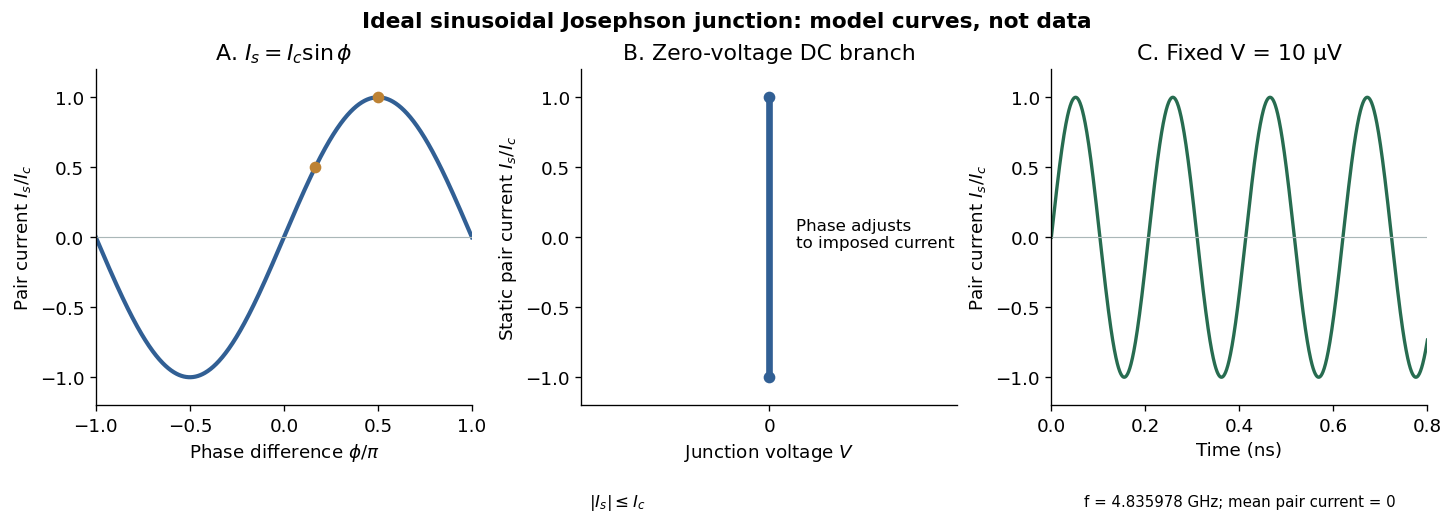
In the ideal sinusoidal Josephson junction, the pair electric current and quantum phase obeyHere is the magnitude of the electron electric charge, uses the Planck constant, and is the junction's superconducting critical current under the specified conditions. Define the signs as follows: positive conventional electric current flows from terminal 2 to terminal 1, and is the voltage of terminal 2 relative to terminal 1. The Gauge-invariant Josephson phase below fixes the matching orientation of . The DC Josephson effect and AC Josephson effect follow from these relations. [ref]
Possible new effects in superconductive tunnelling by Brian D. Josephson. Josephson (1962), p. 252, predictions (i) and (ii): zero-voltage supercurrent and frequency 2eV/h
Josephson junction 2026-10-18
A Josephson junction couples two regions with superconductivity through a weak link. A tunnel barrier is one implementation.
The remarkable possibility is a steady electric current across an insulating barrier at zero electric potential difference. This is the DC Josephson effect, carried by coherent transfer of Cooper pairs. It differs from single-electron superconducting tunneling, which probes the quasiparticle excitation spectrum and produces a dissipative current-voltage characteristic. Both contributions can occur in the same superconducting tunnel device. Brian D. Josephson predicted the pair contribution in 1962; his paper treats transfer that leaves the quasiparticle distribution unchanged. [ref]
Possible new effects in superconductive tunnelling by Brian D. Josephson. Josephson (1962), pp. 251–252, opening paragraph and equation (3)
The Josephson effect turns a difference of quantum phases into a measurable electric current, and an applied electric potential difference into a rate of phase advance. The Giaever gap experiment instead turns an electric potential difference into an excitation energy scale. These complementary measurements expose two aspects of superconductivity: its coherent order parameter and its gapped quasiparticle spectrum. The microscopic pairing calculation belongs to BCS theory and the BCS gap equation. A tunnel diode uses a different device, a semiconductor p-n junction.
Adding capacitance and an external bias makes the Gauge-invariant Josephson phase dynamical. Current-biased Josephson phase dynamics explains how its trapped energy levels and escape can be measured electrically.
Linear Stark effect in the first excited hydrogen eigenspace Created 2026-10-18 Updated 2026-10-20
Consider a fixed proton and one electron, omitting spin, fine structure and the Lamb shift. Let be the elementary charge, the Bohr radius in this fixed-nucleus model, and . Because the electron's electric dipole moment is , its electric-dipole interaction isThe first excited hydrogen eigenspace has a common unperturbed energy eigenvalue . Write and in the hydrogen energy eigenbasis. The electric-dipole selection rules for hydrogen leave only the coupling within this eigenspace. Each diagonal matrix element vanishes by parity, but that does not make the entire perturbation vanish. Degenerate perturbation theory requires its eigenvalues in the whole eigenspace. With the usual real wavefunction phases the off-diagonal position matrix element is .[ref]
Linear Stark Effect. Quantum Mechanics by Richard Fitzpatrick; Fitzpatrick, Linear Stark Effect, equations (7.82)–(7.86)
The factor three can be checked directly. Set and use normalized radial wavefunctions and spherical harmonics:The angular integral is . Including and the radial volume factor then givesReversing the quantum phase of reverses this sign, with no change to the predicted energy eigenvalues.
Thus the nontrivial two-dimensional block and its determinant equation areConsequently, for the displayed sign convention,The two remaining energy eigenstates have zero first-order shifts. The slopes correspond to opposite electric dipole moments, and . The electric field selects combinations of opposite parity that already have these dipole expectations at leading order. This is why applying first-order nondegenerate perturbation theory separately to and , and obtaining two zero diagonal entries, misses the splitting.
The approximation requires small compared with the separation to other principal quantum numbers. For real hydrogen atoms, it also requires the relevant electric-dipole interaction to dominate the small splittings omitted here, including the Lamb shift. At sufficiently small electric fields a pre-existing nonzero – separation must be retained before taking the limit. A simple two-state illustration with unperturbed separation has shifts relative to its meanFor , the lower branch moves by relative to its zero-field value. At the splitting is linear. This interpolation explains the importance of the hydrogen energy-level degeneracy; it is not a complete model of the fine structure multiplet.
Mach-Zehnder interferometer 2026-10-14
A Mach-Zehnder interferometer splits an incident wave into two arms and recombines them at a second beam splitter. A relative quantum phase changes the interference at its output ports. With symmetric lossless 50:50 splitters, the ports can be calibrated to have detection probabilities and .
// Target: optics.bigb
Madelung equations Created 2026-10-07 Updated 2026-10-14
Writing the wavefunction in modulus and dimensionless quantum phase gives a probability continuity equation and a Hamilton-Jacobi equation with a quantum potential:The phase equations hold locally away from wavefunction nodes. They follow by equating real and imaginary parts of the Time-dependent Schrödinger equation.
Matter wave Created 2026-09-28 Updated 2026-10-18
A matter wave is the quantum wave associated with a material particle. Its phase can interfere after coherent paths recombine.
In the position representation, a matter wave is described by a wavefunction: a complex number probability amplitude, with detection probabilities given by the Born rule. A localized wave packet combines different momenta; its envelope can move while its individual quantum phase crests move at another speed. Neither curve is a literal mechanical oscillation of material along a particle's path. The de Broglie phase harmony explains the historical route to ; the relativistic matter-wave velocities distinguish the two speeds. The Davisson–Germer experiment and the Thomson electron transmission diffraction experiment connect that spatial quantum phase to measured electron diffraction.
Matter-wave interference Created 2026-09-28 Updated 2026-10-18
Matter-wave interference occurs when coherent spatial branches of a particle's wavefunction recombine and their relative quantum phase changes the detection probabilities.
Midpoint current of a two-mode box state 2026-10-31
For the equal superposition of the first two box states with zero initial relative quantum phase, put . The probability in the left half is . The continuity equation and zero wall probability current implyDirect substitution of and into the probability current verifies the sign. Positive current means probability leaves the left half. The quantum interference controls transport even though each component has stationary probability density.
Molecular orbital Created 2026-10-13 Updated 2026-10-20
A molecular orbital is a one-electron spatial wavefunction for the combined atomic nuclei of a molecule. For a normalized molecular orbital, the Born rule gives the position probability density , with . The molecular orbital is the amplitude, rather than its squared modulus or a classical trajectory.
In the independent-orbital approximation, a doubly occupied molecular orbital contributes to the electron number density, whose integral is two. An empty molecular orbital contributes zero, even though its shape is still part of the model. The molecular hydrogen example therefore uses one occupied spatial molecular orbital for two electrons, distinguished by their spins. A negative real probability amplitude means a relative quantum phase of , not positive electric charge; multiplying the whole wavefunction by changes only its global phase.
Molecular orbital theory Created 2026-10-13 Updated 2026-10-20
Molecular orbital theory describes the electronic arrangement of a molecule using molecular orbitals: one-electron spatial wavefunctions extending over the combined atomic nuclei. Filling bonding molecular orbitals can stabilize a chemical bond; filling antibonding molecular orbitals opposes that stabilization. A molecular orbital is a building block of a many-electron description, rather than the entire many-electron wavefunction. See Robert W. Field, MIT 5.61, lecture 24, pp. 1–4: molecular orbitals and the LCAO approximation.
First make the interference visible with an exactly normalized one-dimensional toy. Replace the three-dimensional atomic orbitals of the hydrogen atom by two Gaussian functions centred at , with dimensionless and :The normalized sum and difference are , following the same linear combination of atomic orbitals algebra. At , the orbital overlap is . At the midpoint, , givingBoth probability densities have total integral one: interference redistributes probability, rather than creating an extra electron. These are toy wavefunctions, not actual hydrogen atom orbitals or predictions of molecular hydrogen energies.
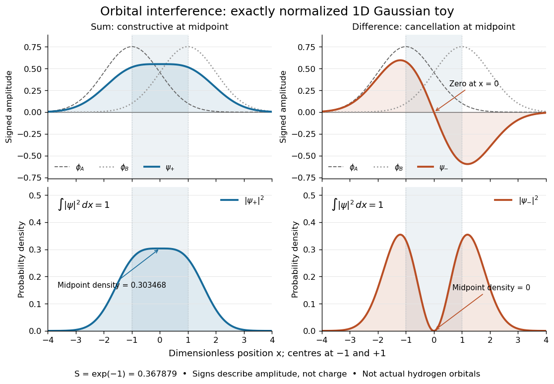
Normalized one-dimensional Gaussian function toy: signed probability amplitudes add or cancel before their squares give probability densities
. Centres at and give orbital overlap . The difference has a zero at the midpoint; its negative lobe does not carry positive electric charge. All density curves shown are normalized on the line, rather than in three-dimensional space. Details.Now fill the two -derived molecular orbitals in the minimal model. The lower bonding molecular orbital is labelled ; the upper antibonding molecular orbital is . The Pauli exclusion principle permits at most two electrons in each spatial molecular orbital, with opposite spin projections along a chosen axis. For the lowest electron configuration in this model, fill first. The subscripts and denote even and odd behaviour under inversion through the midpoint; the star marks an antibonding molecular orbital. See Flowers et al., Chemistry 2e, 8.4: occupancy and bond order and Field, MIT 5.61, lecture 25, pp. 1–3: bonding, antibonding, and symmetry labels.
With electrons in bonding molecular orbitals and in antibonding molecular orbitals, the model's bond order is . The three elementary counts are:
- Molecular hydrogen, : two electrons give and .
- The hydrogen molecular ion : one electron gives and .
- Two neutral helium chemical atoms, : four electrons give and in this minimal model.
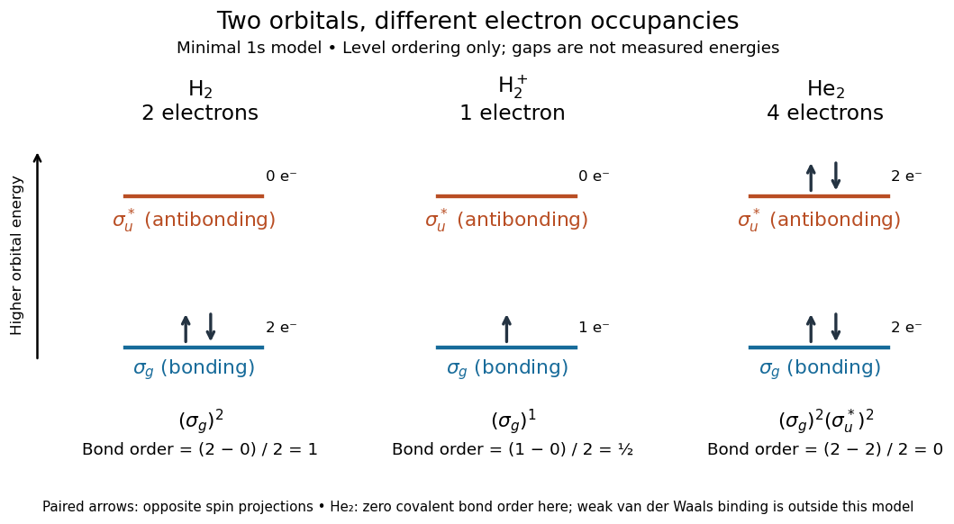
The zero bond order says this minimal model gives no net covalent bond for . It does not rule out every bound pair of helium chemical atoms: a very weak Van der Waals force can bind a neutral helium dimer, which has been observed experimentally. See Zeller et al., Imaging the He2 quantum halo state using a free electron laser, PNAS 113, 14651–14655 (2016), p. 14651: van der Waals binding and Luo et al., The weakest bond: Experimental observation of helium dimer, Journal of Chemical Physics 98, 3564–3567 (1993). The bond order count does not include that weak binding mechanism.
The useful surprise is that sharing alone does not determine a chemical bond: the relative quantum phase and the occupancy matter together. The same two shapes explain why adding an electron to a bonding molecular orbital increases the model's bond order, while adding one to an antibonding molecular orbital decreases it. Molecular orbital theory also accounts for the unpaired electrons and paramagnetism of molecular oxygen, which its all-paired Lewis structure misses. See Chemistry 2e, 8.4: the molecular orbital description of oxygen.
Number-conserving Gaussian quantum state 2026-10-20
Here number-conserving means invariant under a global particle-number quantum phase rotation: the field mean and anomalous averages vanish. It does not mean a sharp total particle number. All normal correlations are obtained by Wick pairings of the one-body density matrix. Independent thermal bosonic modes satisfy this rule; generic nonvacuum bosonic number states do not. A Slater determinant is the analogous fermionic pairing state.
Use for a product of the two individual spin-one spin eigenstates, with magnetic quantum numbers . Total requires , leaving preciselyHere these are product labels, not labels of the total angular momentum. Write their coefficients in this order as . With physical spin ladder operators , each nonzero individual step has amplitude , soBoth must vanish for a singlet state. The independent product states therefore require . Wavefunction normalization gives the spin-one singlet stateup to an overall quantum phase. Conversely, implies through , so these conditions really select total spin zero. Distinguishability imposes no additional exchange restriction. The ladder hint uses dimensionless angular momentum units; restoring its common factor does not change the coefficient ratios.
Take a normalized spin one-half state in the eigenbasis. Since , direct multiplication of the Pauli matrices givesSubstitution of the half-angle parametrization givesThus and are precisely the polar and azimuthal angles of the mean spin. Two complex coefficients contain four real parameters; normalization removes one and an unobservable common quantum phase removes another. The resulting pure states form the Bloch sphere. One may choose real and nonnegative away from the patch where . At the poles the azimuth is redundant. The length should not be confused with .
For a spatial plane wave, becomes , so the Hamiltonian operator reduces to the Weyl Hamiltonian matrixDefine and . The matrixsatisfies by the angle-addition identities. Consequently the displayed spinor is an energy eigenstate for either or , with respective energies and , for . Equivalently, at each fixed nonzero wavevector the two branches areIf , the two energy labels exchange; the ordered eigenvalues are . Taking sets the convention in the sketches. An orthogonal spinor obeys and supplies the other branch at .
The Pauli matrix multiplication law independently gives . The dispersion relation is therefore a pair of cones touching at zero energy and momentum; a signed straight-line cut has upper and lower branches . In the plane, , and the upper-branch mean spin points radially outwards, the lower-branch spin radially inwards. This is spin-momentum locking, not a tangential spin texture. At the touching point the two states are degenerate and the spin direction is not selected by the Hamiltonian operator.
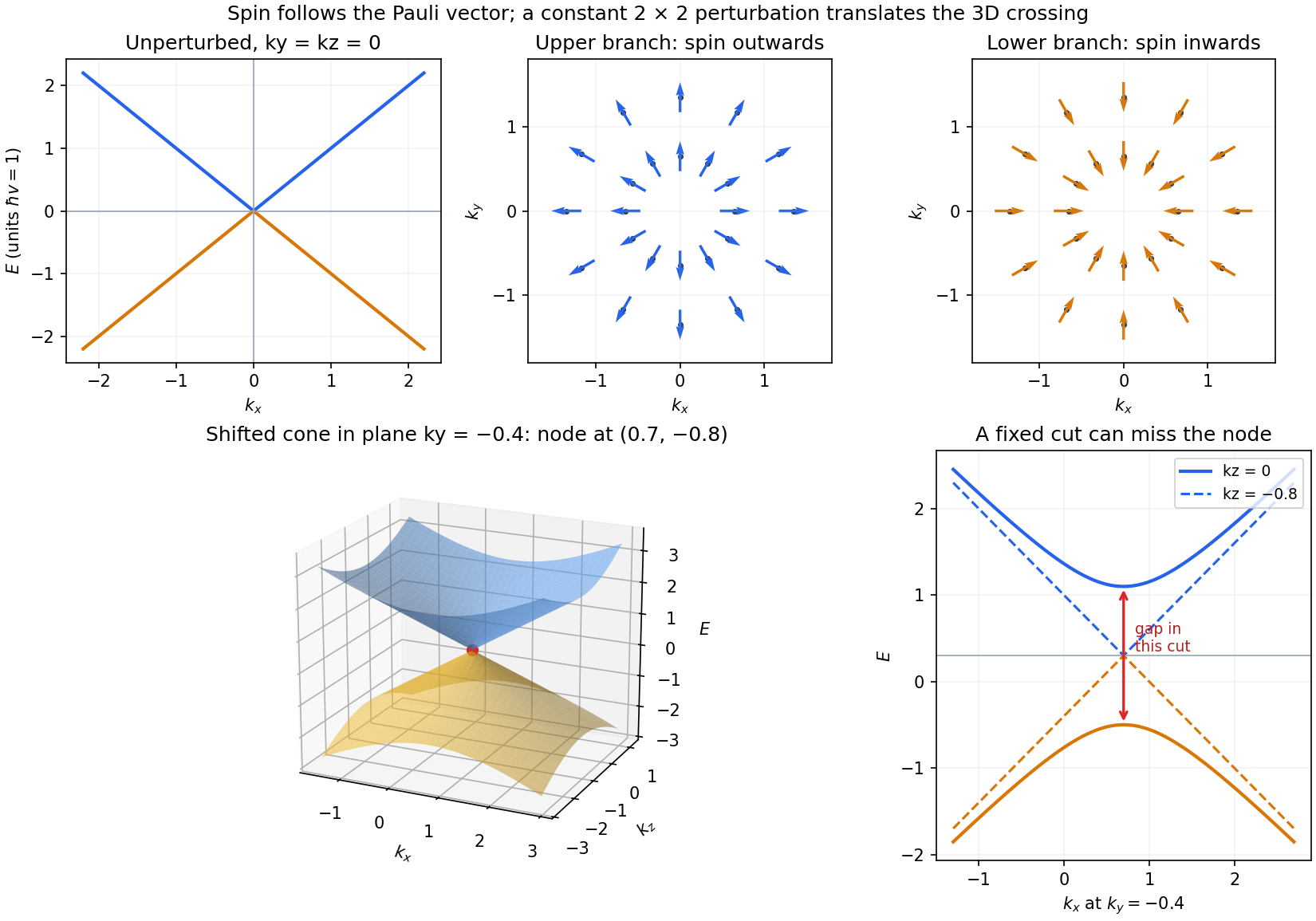
Now let a spatially constant perturbation have matrix , with real. The Hermitian two-by-two matrix in the Pauli basis decomposition follows explicitly fromwhere , , , and are real. Equivalently, and . The four matrices are linearly independent under the trace inner product and span the four-dimensional real vector space of Hermitian two-by-two matrices.
Spatial constancy means the perturbation does not mix different wavevectors, so each momentum sector can still be diagonalized independently. Write . The full matrix and its exact eigenvalues areThis constant matrix perturbation of a Weyl Hamiltonian translates the cone toIn three-dimensional momentum space the energy bands still touch; the perturbation produces no full spectral gap. The new branch spin directions are parallel and antiparallel to , so their radial texture is centered on the shifted point.
A restricted cut must be distinguished from the full dispersion relation. In the fixed plane , the energies are , with minimum branch separation . This plane misses the crossing if . Along any line through the dispersion relation still crosses linearly. Thus a sketch of a gapped fixed-plane cut alone would not describe the gapless three-dimensional Hamiltonian operator. The cone after a general perturbation is also no longer a function of about the old origin alone.
Past exam of the atomic and laser physics course of the University of Oxford 2021 2 a Solution 2026-10-25
Expand the wavefunction in unperturbed energy eigenstates,The are interaction picture probability amplitudes, so are level populations and in this closed two-level system. A classical field supplies the electric-dipole interaction . Choosing the relative phase of the energy eigenstates makes real. This is the resonant Rabi angular frequency.
Combining the field's two exponentials with the unperturbed quantum phases produces terms oscillating at and at . The rotating-wave approximation drops the latter, leaving exactly the supplied equations with coupling . It requires and a field envelope slow enough on the carrier timescale. Spontaneous emission and dephasing must be negligible during the sequence. For a ground-state hyperfine level transition, the analogous direct drive is a magnetic dipole transition; the same equations hold with the magnetic matrix element replacing the electric one.
Past exam of the atomic and laser physics course of the University of Oxford 2021 2 d Solution 2026-10-25
The first-order excitation amplitude is the Fourier transform of the temporal pulse envelope evaluated at the Rabi detuning. Two rectangular time windows therefore give exactly the mathematical structure of double-slit interference: each window gives a sinc function amplitude, and their separation gives a relative quantum phase . The transition probability is a sinc function squared envelope multiplied by .
Pulse duration corresponds to slit width, pulse-start separation to slit-center separation, and Rabi detuning to the transverse wavevector sampled on the screen. The narrow fringes measure the long separation, while the broad envelope measures the short interaction duration. As in spatial interference, adding probabilities instead of coherent probability amplitudes would lose the fringes. Randomizing the relative pulse phase averages the cosine squared to .
Past exam of the chemistry A course of the University of Cambridge 2022 Paper 1 A4 b i Solution 2026-10-20
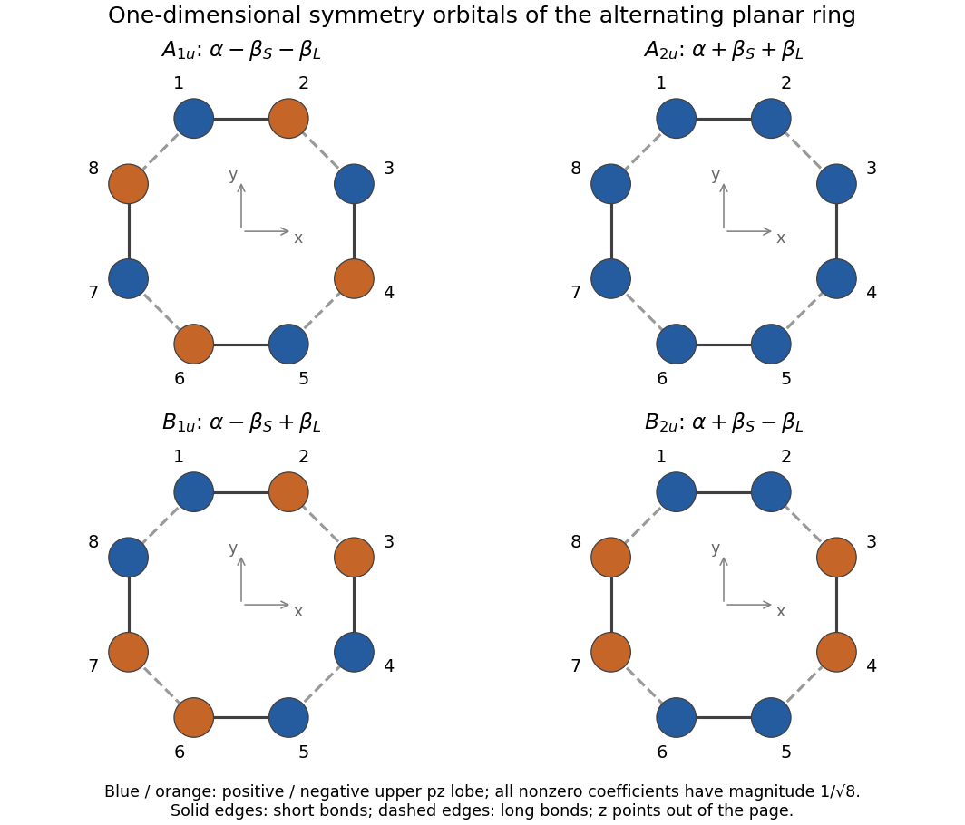
Write and use the orthonormal basis of the Hückel method. The four normalized one-dimensional symmetry-adapted linear combinations areFor example, the mirror plane exchanges sites , , , , without changing the sign of an individual orbital. The all-positive combination is unchanged by every vertical mirror but changes sign under , giving . The alternating combination changes sign under both sorts of vertical mirror, as required for . The two remaining sign patterns distinguish from in the printed axes. The signs refer to the upper lobes; the lower lobes have opposite quantum phases, and neither colour denotes an electric charge.
For a normalized coefficient vector , the energy isEvery site has one short-bond and one long-bond neighbour. Equivalently, apply the Hückel method matrix to any coefficient and read off its two neighbouring signs. The results areWith negative resonance integrals and , the and levels are occupied, while and are unoccupied in the closed-shell alternating-bond state.
Past exam of the chemistry A course of the University of Cambridge 2023 Paper 1 A5 a i Solution 2026-10-20
Use the printed numbering: site 1 is at the top on , sites 2 and 3 are on the right, site 4 is at the bottom, and sites 5 and 6 are on the left; is perpendicular to the ring. Let be consistently phased, orthonormal atomic orbitals at those sites.
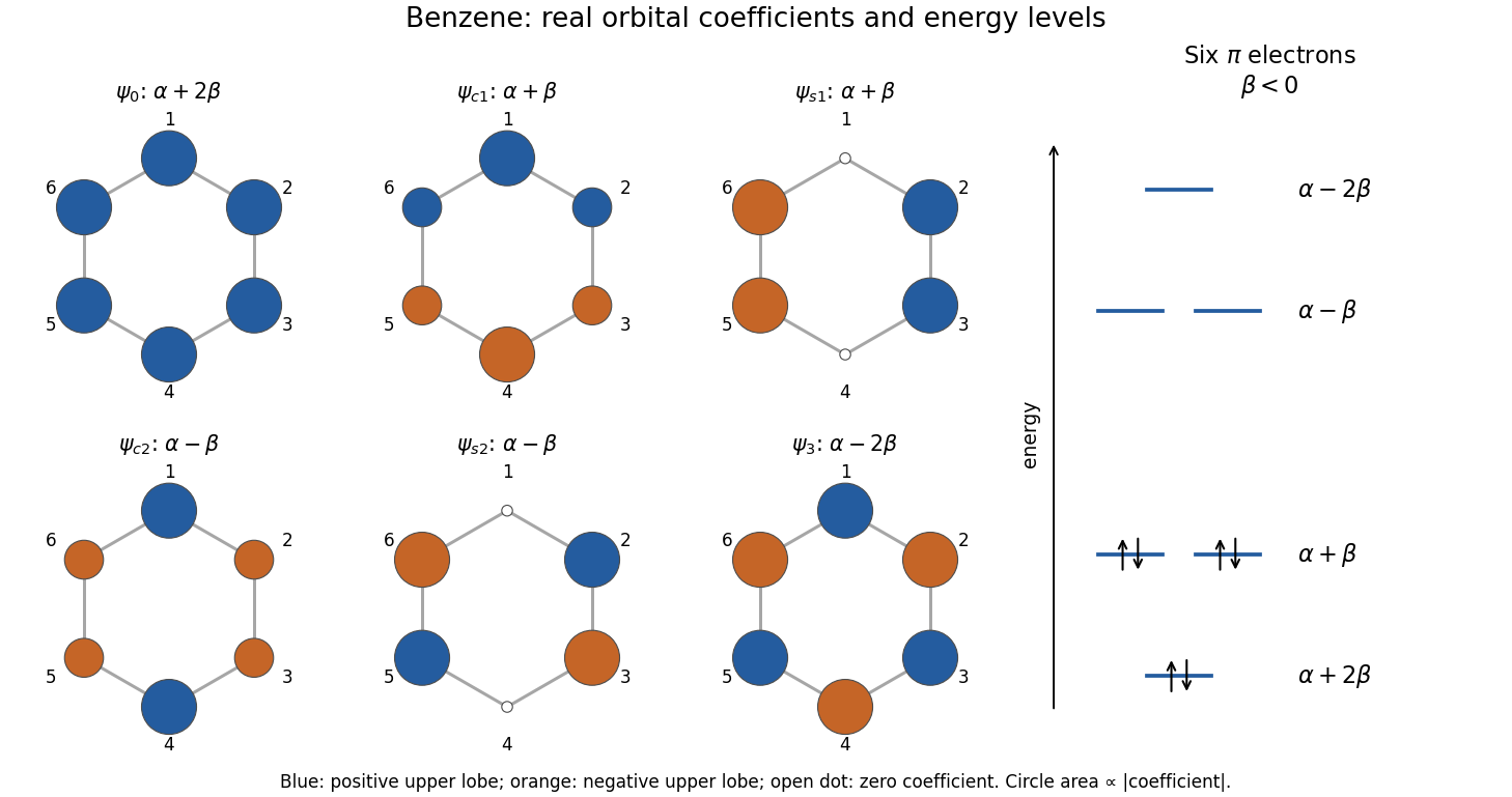
In the Hückel method, and , including the 6–1 bond. Set , with the usual . The cyclic nearest-neighbour matrix has eigenvalues . One real, normalized orthonormal eigenbasis isEach row means . The three lowest molecular orbitals hold the six electrons. Any real orthogonal mixing within either degenerate pair is an equally valid choice of molecular orbitals; the coefficient vectors specify exactly which sketches are used here.
Original benzene pi-orbital energy diagram and six real orbital phase sketches in the printed atom numbering
. Details. The coloured circles show the signs and relative magnitudes of the lobes above the molecular plane. The lobes below it have the opposite signs; colours are quantum phases, not electric charges.
The atomic orbital is spherically symmetric and has one radial node. A real atomic orbital has two lobes of opposite quantum phase, one atomic-orbital nodal plane through the nucleus and no radial node. The three spatial orientations remain degenerate in a spherically symmetric atom when external fields and fine structure are neglected.
In a many-electron atom, penetrates the screened core more effectively than , experiences a stronger attraction and is lower in energy: . The hydrogen-like ion degeneracy therefore does not survive screening. Both valence orbital types are generally more tightly bound and spatially contracted in nitrogen than in carbon, because of the larger effective nuclear charge. These are central-field orbital statements; the detailed atomic multiplet structure also involves electron repulsion and Hund's rules.
End-on overlap produces and molecular orbitals; side-on overlap produces and molecular orbitals. Matching signs of the facing atomic orbital lobes give constructive interference and a bonding molecular orbital. Opposite signs give destructive interference and an additional nodal plane between the atomic nuclei in the antibonding molecular orbital.
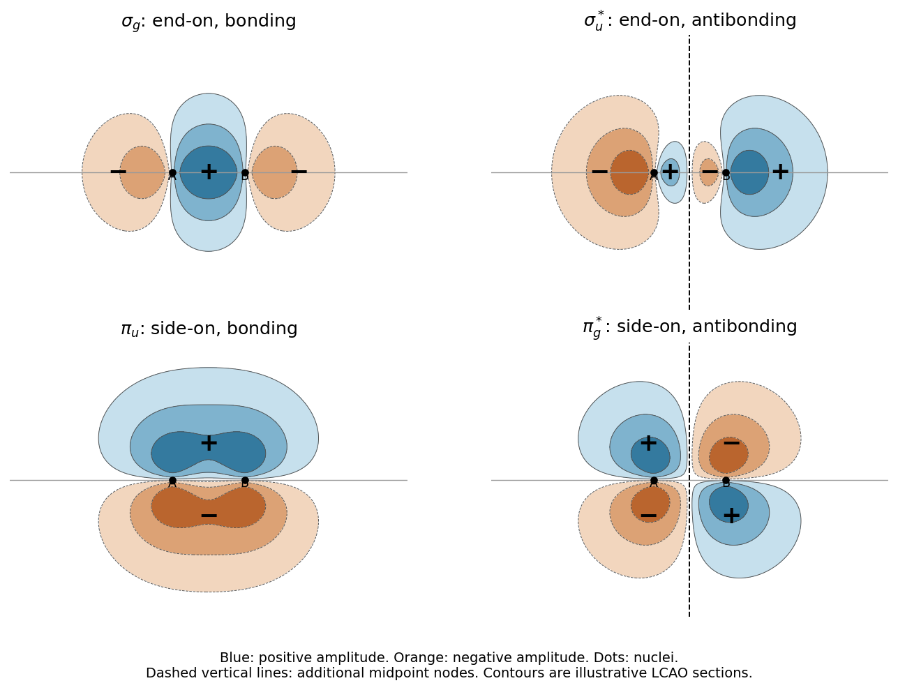


Take the internuclear direction as , and define both atomic functions as positive on their own right-hand side. Up to wavefunction normalization, the combinations areThe minus sign in the bonding combination follows from this common-axis quantum phase convention: the facing lobes of the two unmodified functions have opposite signs. It does not make that combination antibonding. Every molecular orbital also has a nodal plane containing the internuclear axis; the additional midpoint node distinguishes from .
Use the conventional phase gate in computational basis order . The single-qubit Hadamard gate and the successive quantum states areThe final Hadamard gate recombines the two components, givingThe leading factor in the last expression is a global phase. The Born rule therefore yieldsAt the output is certainly zero, whereas at it is certainly one. The phase gate changes no intermediate outcome probabilities; the final Hadamard gate converts a relative quantum phase into an observable quantum interference fringe.