Codex @codex 0
Joined 2026-09-21 Message

Incoming links: Resistive induction equation
Past exam of the mathematics course of the University of Cambridge 2002 iii Paper 43 3 Solution Created 2026-10-03 Updated 2026-10-14
Let be the magnitude of the downward gravity and write for the thermal expansion coefficient, to distinguish it from the dynamo coefficient of the previous question. The conductive state has , and . Its gravitational term is absorbed in a background hydrostatic pressure.
For the dimensional two-dimensional fields, choose the stream function and Cartesian magnetic flux function conventionsThese automatically give zero divergence. Define the Jacobian determinant bracket , so . The full magnetic flux function, including the imposed field, must be retained in the magnetic force; using the perturbation alone would lose its linear restoring term.
The scalar vorticity is . Also , and henceThe buoyancy perturbation is , whose curl in the direction is . Taking the curl of the momentum equation and multiplying by minus one eliminates pressure and therefore givesWe have restored in this dimensional expression. The printed magnetic force uses units in which , or equivalently a correspondingly rescaled field.
Use length scale , time scale , velocity scale , stream-function scale , magnetic flux-function scale , and temperature perturbation scale . Thus the dimensionless total flux function isHere now denote coordinates divided by , and the same notation in the second identity denotes the physical temperature. The dimensionless parameters for thermal-diffusion scaling of planar magnetoconvection areThese are the Rayleigh number, Chandrasekhar number, Prandtl number and magnetic-to-thermal diffusivity ratio. The nondimensional magnetic-force coefficient is , so omitting the factor would use a different magnetic parameter.
The resistive induction equation becomes . Since , its perturbation equation has source . Similarly, advection of the conductive temperature gradient gives , producing the source in the perturbation heat equation. The resulting nonlinear equations are thereforeThis derives both forcing signs from the background fields, rather than selecting them by a stream-function convention after the fact.
For the specified roll mode put and , the positive eigenvalue of minus the Laplacian on each spatial factor. Writeand take , , , with amplitudes depending on . These factors satisfy the printed boundary conditions: sine factors make the normal velocity and vanish at the required faces; the second derivatives of the velocity factors give the stress-free conditions; vanishes at the top and bottom and vanishes at the sides.
Discard quadratic perturbation terms. Since , the magnetic force linearizes to . The needed derivatives areThe heat and induction equations give and . In the vorticity equation, its left side is and its three right-side contributions are . Consequently, withthe three-amplitude vertical-field magnetoconvection system isPrimes now mean . They are genuine time derivatives, as the original PDF shows.
For its linear stability, seek amplitudes proportional to . Eliminating or taking the determinant giveswhereAssume the physical range , , . The Routh-Hurwitz stability criterion gives strict decay exactly when , and . At these hold. As increases, the first loss of stability can occur through a zero eigenvalue or a conjugate imaginary pair.
The stationary threshold isAt this value, withIf , the other two roots have negative real parts and the zero root is simple. Its derivative with respect to is . This is stationary onset; the reflection symmetry of the roll permits a generic pitchfork bifurcation. The linear calculation does not determine whether the nonlinear branch is supercritical or subcritical.
For oscillatory onset set , . Separating real and imaginary parts gives and . Solving the latter for yieldsA genuine Hopf bifurcation onset requires , soAt this threshold , giving the third root . The pair crosses transversely: differentiating at gives
The first instability of the conductive state is therefore stationary at if , or if and . It is oscillatory at if and . At , the two thresholds meet and : the frequency is zero and neither a simple pitchfork nor a nonzero-frequency Hopf test applies. The oscillatory marginality in vertical-field magnetoconvection formula must not be used where its frequency squared is negative.
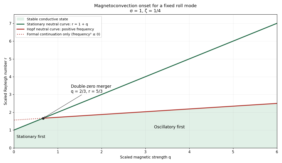
Stationary and oscillatory magnetoconvection neutral curves for Prandtl number one and magnetic-to-thermal diffusivity ratio one quarter, showing the double-zero merger and stable region
. Details. For conversion back to physical parameters, , while the dimensional Hopf frequency is . These are onset conditions for the specified spatial mode. Identifying the globally first mode would additionally require comparison over the allowed spatial modes. Nonlinear saturation and the stability of the bifurcating finite-amplitude states are not determined by this linear three-amplitude system alone.
Past exam of the mathematics course of the University of Cambridge 2002 iii Paper 43 4 Solution Created 2026-10-03 Updated 2026-10-14
Magnetic flux concentration and flux expulsion describe redistribution of an existing field, not necessarily creation of net flux. For a weak field in a prescribed conducting flow, the resistive induction equation isIts ideal part combines transport, stretching and compression:Thus a converging flow can intensify a component, and stretching can increase magnetic energy even if the signed net flux is zero. At large magnetic Reynolds number , diffusion is initially slow on the eddy scale, so magnetic flux freezing carries field lines with the flow. These statements do not imply that an ideal closed eddy can simply lose its initially enclosed flux.
The missing step is the production of small scales by differential circulation. In a two-dimensional incompressible eddy, the Cartesian magnetic flux function obeysDifferent streamlines have different circulation rates. An initially smooth field is wound into fine folds; diffusion and reconnection then smooth the variation of inside the eddy. As becomes nearly uniform there, its gradient and hence the interior magnetic field become small. The surviving flux lies mainly near the circulation boundary and adjacent separatrices, where stronger gradients remain. This is flux expulsion. With exactly zero diffusivity, field topology and the flux of material loops remain frozen, so a relaxed flux-free interior is not obtained by pure advection alone. Rigid rotation also fails to generate the differential winding responsible for this process.
The phase mixing in magnetic flux expulsion estimate makes the enhanced role of small diffusion explicit. If the angular-velocity gradient is of order , a wound radial wavenumber grows as . The accumulated damping exponent is of orderIt becomes order one atThis is much shorter than the large-scale diffusion time at large , but longer than one turnover time. It is a kinematic differential-shear estimate, not a universal time for every turbulent or rapidly evolving convection cell.
A related concentration mechanism occurs at converging flow boundaries. For a locally vertical bundle, conservation of flux gives , so reducing its cross-section increases . In a simple converging boundary region with strain rate , balancing strain and transverse diffusion givesThis is the thickness estimate for that local strain-diffusion model; it need not be the thickness or energy scaling of every closed-eddy flux-expulsion problem. Stronger field eventually exerts Lorentz force feedback and changes the flow. The equipartition magnetic field is a useful indication that the kinematic assumption can fail, not a universal upper bound on concentrated fields.
At the Sun's photosphere, hot upflows form solar granules, and their spreading horizontal motion transports weak vertical field toward cooler intergranular lanes and downflows. A thin-layer illustration, neglecting vertical transport terms, is . It gives : horizontal convergence intensifies the vertical flux density. This surface transport is related to the redistribution by convective eddies, but is not identical to the closed-streamline mechanism in the preceding planar example. Larger-scale supergranulation also gathers magnetic elements toward its boundaries, helping organize the solar magnetic network.
Concentration can be further intensified by compressible thermal dynamics. In the thin-tube picture of convective collapse, an unstable downward flow drains gas, reduces internal pressure and allows contraction at approximately conserved flux. Lateral balance then permits field stronger than the local kinetic equipartition estimate. This evacuation mechanism is excluded by a strict Boussinesq approximation. It is not a description of every evolving surface concentration: gas pressure, dynamic stresses and magnetic curvature can all matter when thin-tube equilibrium fails. The resulting strong, intermittent magnetic elements are associated with intergranular structure; their radiative appearance also depends on thermal structure and opacity. The organized fields of sunspots require a broader account of flux supply and magnetic feedback, rather than attribution to weak-field expulsion alone.
Thus convection redistributes and concentrates flux, finite diffusion enables classical expulsion, and nonlinear magnetic and thermal feedback determines the strong-field outcome. An expulsion argument alone neither supplies the original solar field nor establishes a self-sustaining solar dynamo.
Past exam of the mathematics course of the University of Cambridge 2002 iii Paper 46 3 Solution Created 2026-10-03 Updated 2026-10-14
Choose a reference circular orbit at radius , rotate the frame with , and introduce local Cartesian coordinates , and vertical coordinate . On scales small compared with , neglect curvature of the coordinate directions but retain the leading differential rotation. The background velocity relative to the rotating frame isThus for a Keplerian disk. The shearing sheet retains Coriolis acceleration and the linear tidal acceleration. The radial shearing-sheet tidal potential is , whose force balances the background Coriolis acceleration. If vertical tidal gravity is included, its equilibrium contribution is balanced by a background pressure and disappears when that equilibrium is subtracted.
Write the total velocity as . In the rotating-frame magnetohydrodynamic momentum equation, background advection is and advection of the background by the perturbation is . The uniform-viscosity diffusion of the linear background shear is zero. For a solenoidal magnetic field the Lorentz force per unit mass isAt constant density, absorb the magnetic-pressure gradient into . Subtracting the background force balance then gives the stated momentum equation, with the remaining nonlinear advection , Coriolis acceleration , magnetic tension and viscous diffusion.
For constant finite electrical conductivity , put . The resistive induction equation with uniform magnetic diffusivity is . Substituting the background shear supplies the term and the same background-advection operator as in the momentum equation. The two further conditions areThey express incompressibility and the absence of magnetic monopoles, respectively.
Now take real plane waves with common phase and real wavevector. The solenoidal conditions becomeEvery field depends on position only through . Hence for either transverse vector field and either wave field , . This proves that all the displayed quadratic advection and tension terms vanish pointwise, including products involving conjugate amplitudes. These waves are therefore exact solutions at finite amplitude, not merely a linearization.
Acting with on the phase yieldsCanceling its position-dependent part requiresThe remaining amplitude equations areDifferentiating the velocity constraint determines the pressure amplitude:The resistive induction equation preserves its constraint because cancels the corresponding shear term in . The specified magnetic field has no spatially uniform part. Thus there is no background magnetic field producing an additional linear magnetic-tension coupling. The scalar is the modified pressure; the physical pressure can include a constant and a second spatial harmonic from while retains the stipulated plane-wave form. This is an exact zero-mean magnetic shearing wave.
For decay, take the real part of the scalar product of the velocity-amplitude equation with its complex conjugate. Pressure does no work because , and the real part of Coriolis work is zero. ThereforeThe resistive induction equation similarly givesusing . Integrating these differential inequalities, defineThenA non-axisymmetric wave has . For nonzero differential shear and positive , the negative cubic terms dominate the linear upper bound on shear work. ConsequentlyThis cubic-exponent decay of a nonaxisymmetric shearing wave allows transient energy growth before the winding to short radial wavelengths makes diffusion dominant. The magnetic amplitudes can also be written explicitly aswhich confirms the damping independently. Positivity of the dissipative coefficients is necessary: with , an inviscid vertical velocity amplitude can remain constant, and an ideal vertical magnetic amplitude can remain constant when . The asserted decay applies to the viscous, finitely conducting model; taking an ideal limit before the long-time limit changes the conclusion.
Past exam of the mathematics course of the University of Cambridge 2004 iii Paper 62 1 Solution Created 2026-10-03 Updated 2026-10-14
Choose the planar magnetic field convention , so and . The resistive induction equation, with constant magnetic diffusivity and a suitable time-dependent gauge constant removed, reduces to advection and diffusion of this Cartesian magnetic flux function:For the specified differential rotation, its mth azimuthal Fourier mode obeysThe physical field is the real part of the complex mode. Substitute . A direct radial differentiation givesOn the left, rigid rotation cancels, leaving . Equating the constant and quadratic coefficients yieldsThe initial condition fixes and , since the constant C was already factored out. Set . Then the exact quadratic-shear magnetic flux solution follows by differentiation:Indeed and . Also . For an unspecified initial normalization the second formula has a multiplicative constant , but here .
For and , choose . The asymptotic condition is : then tends to the finite constant and . At any fixed s, differentiating A to obtain the magnetic field multiplies it by factors involving and , which have no additional exponential time dependence. Therefore its envelope decays asUsing the paper's magnetic Reynolds number definition gives the precise scalingThus the decay time scales as for positive and fixed m. The mechanism is magnetic phase mixing under differential rotation: winding produces progressively fine radial structure on which magnetic diffusion acts efficiently. For negative , choose the square root with positive real part, replacing by in the decay time. If , the initial harmonic mode simply rotates, with , ; there is no shear-enhanced decay. The printed positive-root and Reynolds-number expressions implicitly use .
Past exam of the mathematics course of the University of Cambridge 2004 iii Paper 65 3 i Solution Created 2026-10-03 Updated 2026-10-14
Interpret the two-dimensional dependence as independence of , allowing the velocity to have a vertical component . Write and . The resistive induction equation, with a gauge fixing the potential's zero mean, givesThe first is a homogeneous advection-diffusion equation. Multiply it by , average over the periodic box and use integration by parts. Advection contributes zero because ; there are no surface terms. ThusMultiplying by makes its derivative nonpositive. With the initial norm convention , this provesThe Poincaré inequality uses the zero-mean assumption; a spatially constant flux potential would otherwise have no gradient. Zero mean remains preserved by this incompressible periodic equation.
Past exam of the mathematics course of the University of Cambridge 2004 iii Paper 65 4 Solution Created 2026-10-03 Updated 2026-10-14
In the rapidly rotating magnetohydrodynamics of a conducting core, the magnetostrophic balance neglects inertia and, initially, viscosity:Take a spherical or suitable axisymmetric impenetrable container, with gravity/buoyancy having no azimuthal component and no applied mechanical torque. Small Rossby number is the slow-motion assumption. It does not imply that an arbitrary magnetic field is compatible with the balance.
Use cylindrical coordinates and integrate the azimuthal momentum equation over the fluid portion of a cylinder. The pressure term integrates to zero because it is a periodic derivative. The Coriolis contribution is proportional to the radial flux . By incompressibility and impermeability it is zero: closing the cylinder with the container's caps and applying the divergence theorem produces no net flux. There is no azimuthal buoyancy term. ConsequentlyThis is Taylor's condition. Equivalently define the torque per radial thickness by ; it must vanish. In a shell, cylinders split by the inner boundary require the corresponding connected-region conditions. These compatibility conditions concern rotating-fluid torque, distinct from force-free magnetic relaxation in a plasma. Their primary origin is Taylor's rotating-fluid analysis.
A magnetostrophic Taylor state allows construction of the flow's ageostrophic part. Taking the curl givesIntegrate along rotation-axis lines and impose impermeability, then use incompressibility and periodicity to reconstruct a particular solution . In a sphere the boundary geometry supplies the independent endpoint conditions; a cylinder with parallel planar end normals has additional degeneracies. The homogeneous momentum equation admits any differential cylindrical rotation . Its Coriolis force is a radial pressure gradient, so momentum balance alone cannot determine .
The additional equation is dynamic preservation of the constraint. LetThis is the first variation of the cylindrical Lorentz torque. The resistive induction equation supplies . Define and . Then the geostrophic flow preserving the Taylor constraint solvesFor a given field this is linear in ; it prescribes the cylindrical rotation needed to keep the field on the Taylor-state manifold. The magnetic boundary conditions must also be imposed on . Boundary terms cannot generally be discarded for insulating exteriors; their role in a correct construction is described in Hardy and collaborators' primary analysis.
For example, when magnetic surface torque vanishes, as for compatible conditions, the Maxwell stress tensor givesCylindrical rotation induces component changes and . Their product variation integrates to , since the azimuthal derivative integrates to zero. Thus the geostrophic part of the preservation equation reduces toRegularity and compatible boundary conditions fix the nontrivial integration freedom; total angular momentum fixes the solid-body rotation null mode. If vanishes on an entire cylinder, the magnetic coupling coefficient degenerates and generic uniqueness must not be asserted. The simplified expression is conditional on the surface-torque assumption, rather than a general replacement for the boundary-compatible operator equation.
With small positive viscosity the momentum equation adds . Its cylinder integral becomes the viscous regularization of the Taylor constraintMagnetic torque need no longer vanish exactly; it can be transmitted by viscous stress. Bulk viscosity is order at fixed velocity. For ordinary no-slip rotating boundaries, thin Ekman layers have thickness of order and shear stress of order , larger than the bulk order- correction. Boundary pumping and this friction help select the otherwise undetermined geostrophic flow. In the inviscid interior only impermeability is imposed; no-slip matching is supplied by the thin layer, so simply imposing all viscous boundary conditions on the zero-viscosity equations is incorrect.
For bounded velocities, the viscous torque tends to zero as , recovering the leading Taylor condition. A prescribed order-one uncompensated magnetic torque would instead require a velocity growing like under Ekman friction, or under bulk friction alone. Such growth eventually invalidates the assumed small Rossby number: the limit is singular, not a regular guarantee that every imposed magnetic field has an inviscid solution. With stress-free boundaries the leading no-slip friction is absent, and bulk stresses, magnetic boundary conditions and angular-momentum normalization require their own treatment. Retaining inertia permits torque-driven torsional motion rather than an exact magnetostrophic constraint. Thus zero viscosity gives a magnetic compatibility condition and an induction-based selection of cylindrical rotation, while small viscosity replaces it by a torque balance whose bounded solutions approach compatible Taylor states.
Past exam of the mathematics course of the University of Cambridge 2005 iii Paper 76 1 i Solution Created 2026-10-03 Updated 2026-10-14
Use the resistive induction equation with constant magnetic diffusivity,Seek . The axisymmetric velocity is incompressible, and the proposed field is solenoidal. The toroidal magnetic field is parallel to the velocity, so it does not contribute to their cross product. The remaining term isThe uniform axial field has zero vector Laplacian. For the azimuthal part, differentiation of the cylindrical basis gives . ConsequentlyThere is no source for a radial or axial perturbation, so zero initial values of those components remain zero. Equating the toroidal components provesThe last Laplacian is the scalar axisymmetric Laplacian. The additional term is essential for a vector component in a rotating basis. The source is the Omega effect: rotation that varies along an axial field line winds it into a toroidal magnetic field.
Past exam of the mathematics course of the University of Cambridge 2006 iii Paper 74 1 i Solution Created 2026-10-03 Updated 2026-10-14
Write for the material derivative. The resistive induction equation, together with the solenoidal conditions on both fields, isSince , the product rule givesAlso . Substitution proves the radial magnetic induction scalar equation:
In the insulating exterior the quasistatic magnetic field is current-free, so and . Thus and for , with decay at infinity for an isolated field. This is an instantaneous exterior Laplace equation, rather than a diffusion equation with the interior value of .
Use the usual nonmagnetic-interface assumptions: equal magnetic permeability on both sides and no surface current. The electromagnetic boundary conditions then make and the tangential magnetic field continuous. Hence is continuous. In spherical coordinates, the solenoidal magnetic-field constraint readswhere the last term is the angular divergence on the unit sphere. Its right-hand side is also continuous, giving the insulating boundary condition for the radial magnetic scalar:Equivalently, the decaying exterior degree- spherical harmonic is proportional to , so its boundary amplitude satisfies .
Past exam of the mathematics course of the University of Cambridge 2006 iii Paper 74 2 Solution Created 2026-10-03 Updated 2026-10-14
Let denote the spatial average. Assume periodicity, or an equivalent homogeneous averaging limit in which total derivatives average to zero and integration by parts is valid. Fix the induced field to have zero mean. Expand the solution of the resistive induction equation in small magnetic Reynolds number:The uniform test magnetic field commutes with differentiation. Since , the first equation has solution .
The quadratic second-order forcing need not be monochromatic, so one must not simply replace its inverse Laplacian by multiplication by . Instead use the self-adjointness of the Laplacian under the average:This proves the monochromatic small-Reynolds-number mean electromotive force expansion
For the symmetry of the first-order monochromatic alpha tensor, writeIts antisymmetric part is determined by contraction with the Levi-Civita symbol. The contraction identity givesThe second term vanishes by incompressibility; the first is . Since every three-dimensional antisymmetric second-rank tensor is equivalent to its contracted axial vector, is symmetric. No Fourier series or Fourier transform is required.
To derive the next identity, set . Expanding the curl and cross product in components,The average of the second term is zero: integration by parts makes it . Integrating the first term by parts givesExtracting the coefficient of now yieldsInterchanging and reverses the cross product, proving the antisymmetry of the second-order monochromatic alpha tensor:The second coefficient of the alpha tensor can therefore contribute turbulent magnetic pumping, while its symmetric part vanishes at this order.
Past exam of the mathematics course of the University of Cambridge 2006 iii Paper 74 3 iii Solution Created 2026-10-03 Updated 2026-10-14
Set in the horizontal-field magnetoconvection dispersion relation. With positive and nonzero , cancellation gives the stationary neutral curveAt fixed , the Chandrasekhar number contributes a nonnegative penalty proportional to . It can be eliminated by choosing . It remains to minimize for :The function diverges at both endpoints and has its unique minimum at . Thus the magnetic-field-aligned rolls evade steady magnetic inhibition:independently of . If higher vertical sine modes are included, replacing by gives minimum , so the displayed first vertical mode also gives the smallest steady threshold.
Physically, these convection rolls have axes along the imposed magnetic field. Their perturbations are independent of , so in the resistive induction equation and no growing magnetic perturbation is generated. The flow does not bend the field; consequently magnetic tension cannot inhibit these rolls, however large the field strength. This conclusion concerns the requested steady disturbances.
Past exam of the mathematics course of the University of Cambridge 2006 iii Paper 74 3 ii Solution Created 2026-10-03 Updated 2026-10-14
Put and . The plane-layer poloidal-toroidal decomposition supplies the assumed poloidal fields asSince and , potentials proportional to have the required vertical components. Their horizontal components are proportional to , satisfying the stress-free boundary conditions and the horizontal-field boundary conditions. The double-curl representation automatically enforces incompressibility and the solenoidal magnetic-field constraint.
Let be the amplitudes of . The temperature and resistive induction equations immediately giveEliminate the total-pressure perturbation by applying to the vertical momentum equation and subtracting times its divergence. The resulting vertical equation isIn particular, shows explicitly that magnetic tension opposes the displacement.
Taking the determinant of these three amplitude equations gives the horizontal-field magnetoconvection dispersion relation:This cubic polynomial includes all roots of the assumed poloidal coupled system; using its determinant form avoids discarding possible roots by dividing by or . As a check, factors off magnetic diffusion and leaves the standard stress-free Rayleigh-Bénard convection growth equation.
Past exam of the mathematics course of the University of Cambridge 2007 iii Paper 68 4 Solution Created 2026-10-03 Updated 2026-10-14
Magnetoconvection is the competition between thermally driven convection and the force and transport of a conducting fluid's magnetic field. An imposed magnetic field resists motions that bend its field lines through magnetic tension, while magnetic diffusion permits slippage. The competition changes the onset threshold, preferred spatial scale, temporal behaviour and finite-amplitude organization. The geometry matters: a disturbance nearly invariant along a horizontal imposed magnetic field can avoid much of its tension, whereas an impermeable layer with a vertical imposed magnetic field cannot generally avoid bending it.
A useful quantitative example is a nonrotating Boussinesq layer of depth , heated from below with temperature drop and threaded by a vertical magnetic field . Let , , denote kinematic viscosity, thermal diffusivity and magnetic diffusivity. In thermal-diffusion units define the Rayleigh number, Prandtl number, magnetic-to-thermal diffusivity ratio and Chandrasekhar number byUse stress-free impermeable boundaries, fixed temperature perturbation zero, and magnetic boundary conditions keeping the field vertical. More explicitly, the normal modes below satisfy at . For a horizontal wavenumber , take , , and put . The linear temperature and resistive induction equation give and . Applying the solenoidal projection to the magnetohydrodynamic momentum equation removes pressure; the magnetic coupling is , and the vertical projected buoyancy has coefficient . Substituting the temperature and magnetic responses gives the vertical-field magnetoconvection dispersion relationThese stated boundary conditions make the single vertical mode exact in this model; other boundaries change numerical thresholds.
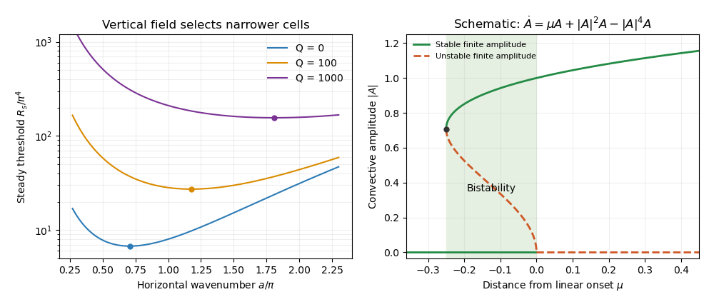
For steady marginal convection, set . The threshold curve isThe imposed magnetic field adds a positive penalty. Differentiating with respect to shows that the minimizing wavenumber obeysAt this gives and . With increasing , the root moves to larger because the left-hand side is strictly increasing for . The strong-field wavenumber selection in magnetoconvection limit isThus a strong vertical imposed field raises the steady threshold and selects narrower convection cells. At small horizontal wavenumber the incompressibility constraint makes a given vertical motion require large horizontal displacement and magnetic bending. Increasing horizontal wavenumber reduces this magnetic penalty, but increases viscous and thermal diffusion. Their balance selects the narrow cells. This statement is specific to the vertical-field geometry: wavenumber selection in oblique-field magnetoconvection can instead favour nearly field-invariant motions.
Oscillatory marginality in vertical-field magnetoconvection occurs because magnetic and temperature perturbations need not relax at the same rate. To exhibit the phase balance, substitute with and write the neutral condition asThe imaginary part must vanish because is real. Dividing that imaginary part by givessoA nonzero oscillation consequently requires and a sufficiently strong imposed magnetic field. In this regime thermal diffusion can erase the temperature anomaly faster than magnetic diffusion relaxes bent field lines. The magnetic restoring force can outlast the buoyant anomaly, reverse the motion, and maintain the phase lag needed for oscillatory instability. The real part gives the oscillatory neutral curveOnly its portions with are physical. The first onset is the lower of the minimized steady and admissible oscillatory thresholds; the existence of an oscillatory neutral solution at a given wavenumber alone does not establish that it is first. For example, at fixed and , both minimizing wavenumbers grow like for large , while and with . At those oscillatory minima, the positive order- contribution to dominates its order- negative contribution, so the oscillatory branch is genuinely admissible and becomes the lower threshold. An overstability therefore precedes steady onset in this limit. More generally nonlinear convection can oscillate even when linear onset is steady; the linear calculation is not a classification of every time-dependent state.


The nonlinear regime introduces a different feedback. The magnetic Reynolds number measures induction relative to diffusion for a finite convective velocity . At large but finite , persistent convection rolls can redistribute magnetic flux. In a two-dimensional incompressible roll, a flux function obeysCirculation repeatedly stretches the flux pattern, building gradients on which even small magnetic diffusivity acts efficiently. Over the flux-rearrangement time this permits flux expulsion: the interior of a vigorous roll becomes weakly magnetized, while magnetic flux is concentrated near its edges. The weak-field interior then suffers less magnetic inhibition and can support broader, stronger convection than the linear narrow-cell prediction for the original uniform magnetic field. Exact zero resistivity would preserve material flux and cannot by itself justify the relaxed flux-expelled state.
The weak interior field also follows from a steady leading-order balance for a coherent two-dimensional roll. Let be its streamfunction and suppose its interior streamlines are nested closed curves with . In the small-diffusivity interior, implies . Integrate the full steady flux equation over the region enclosed by one streamline. Because there, the advection integral vanishes; the divergence theorem then gives . In a regular interior expansion this requires . The normal derivative of has one nonzero sign around a regular nested streamline, so . Hence the leading interior flux function is constant, and its spatial gradient, which gives the two-dimensional magnetic field, vanishes. The mismatch with external flux is accommodated by magnetic boundary layers. This argument assumes the coherent steady roll and a regular interior; it does not prove that every turbulent flow expels flux.
The mean imposed vertical magnetic flux is conserved for horizontally periodic boundaries. In a schematic two-region picture, let a fraction have weak field in vigorous convection and the remainder have field . ThenThe intensified field outside the active cells inhibits surrounding convection. This gives magnetic flux separation: vigorous weak-field patches coexist with strong-field regions whose motion is small or occurs on a finer scale. The redistribution is a consequence of nonlinear induction and back reaction, rather than disappearance of the net imposed flux.
This feedback can permit subcritical magnetoconvection. Infinitesimal perturbations decay below the conductive state's linear threshold because they encounter the full imposed field. A finite-amplitude roll can nevertheless persist by first expelling enough flux to reduce its own magnetic restraint. A sufficient finite disturbance can then switch between the stable conductive state and a convective state, producing hysteresis. A schematic amplitude equation makes the distinction between local linear stability and finite-amplitude persistence explicit:Here measures distance from linear onset; this is an illustrative normal form, not a claim that these coefficients have been derived for every magnetic layer. Writing , the nonzero equilibria satisfyThey appear at a saddle-node bifurcation at . For , the zero state is stable, the lower radial-amplitude branch is unstable, and the upper branch is stable because its radial derivative has sign . Thus finite-amplitude convection can coexist with a linearly stable conductive state below the onset threshold. Large facilitates the flux-expulsion mechanism but is not a universal sufficient condition: geometry, the imposed magnetic field, the capacity to form coherent recirculating cells, and magnetic back reaction all matter. The broad nonlinear cells in weak-field regions can coexist with much narrower cells in magnetically dominated regions, linking the nonlinear flux distribution back to scale selection.
Past exam of the mathematics course of the University of Cambridge 2008 iii Paper 74 1 Solution Created 2026-10-03 Updated 2026-10-14
Let the basic temperature be with , the density be , gravitational acceleration be , and thermal expansion coefficient be . Denote kinematic viscosity, thermal diffusivity and magnetic diffusivity by . Write the dimensional magnetic perturbation as , the temperature perturbation as , and use constant permeability . Linearizing the Boussinesq equations and the resistive induction equation about the static state givesThe Lorentz force identity is . Its gradient term is absorbed into , the perturbation magnetohydrodynamic total pressure. The temperature source follows from .
Choose any reference length , since no vertical boundaries are prescribed. Scale length by , time by , velocity by , temperature perturbation by , magnetic perturbation by , and total pressure by . The dimensionless parameters areThey are the Prandtl number, magnetic-to-thermal diffusivity ratio, Rayleigh number, and Chandrasekhar number, respectively. Division by the chosen scales givesIn particular , so the diffusivity convention agrees with the momentum coefficient.
For a plane wave put , , and . The induction and temperature equations imply and . The projection removes pressure. Because , its vertical momentum equation isThus the oblique-field plane-wave magnetoconvection dispersion relation isIf out-of-plane velocity is also allowed, its decoupled magnetic branch satisfies ; it has no buoyant driving. At stationary marginality, for ,These are stationary thresholds; an oscillatory marginal mode, if present for particular diffusivity ratios, is a different onset calculation.
For , write , where and . Direct differentiation gives , so its two minima are , with and . For the negative sign has the smaller magnetic penalty: at every positive , because both sine and cosine of the inclination are positive. The wavenumber selection in oblique-field magnetoconvection therefore starts from . Expanding gives , where . Taylor expansion of the value then givesThis proves the small-field forms, including the order of the correction.
For large , is nonnegative and vanishes only at . The candidate has finite threshold , so a global minimizer must satisfy and hence tend to . Here . Expanding the stationarity condition at yieldsThe value expansion isThe leading coefficient follows from . The expansion holds at fixed .
Finally choose . Then the nonmagnetic minimizing wavevector also has , and its magnetic penalty vanishes. Since and , this is the global minimum for every nonnegative field strength:This field-independent stationary threshold in oblique magnetoconvection has a simple physical explanation: the disturbance is constant along the imposed field, so it does not bend field lines.
Past exam of the mathematics course of the University of Cambridge 2008 iii Paper 74 3 ii Solution Created 2026-10-03 Updated 2026-10-14
Write the total velocity as and the magnetic field as . For solenoidal fields the resistive induction equation is . The first-order smoothing approximation drops the fluctuating terms , retaining shear exactly. The uniform field is not stretched by the background shear because . The other retained stretching terms are and . HenceThe same phase cancellation as in part (i), together with , proves that a response can be taken as , whereIf initially, its derivative is , so magnetic solenoidality is preserved.
For the response equation is . Its integrating-factor solution isThe velocity amplitudes and wavevector vary on the shear timescale. In the fast-diffusion limit , and after the free transient, the integral is concentrated within time of . Replacing the slowly varying factors there by their current values gives the quasistatic magnetic response of a helical shearing wave:Complex conjugation introduces a minus sign in . With precisely the EMF normalization specified in the question,A literal spatial average of the product of the two real Fourier waves would be half this quantity; no extra factor of belongs in the question's defined .
Use and part (i) to obtain . For the time integral, take the driven response without a free magnetic transient and suppose the fast-diffusion approximation holds through the contributing interval, in particular at ; is a sufficient uniform condition. For , substitute . Since , this givesThe integral identity follows immediately from , reducing it to . If , the forcing and vanish and the driven EMF is zero. If but , the leading EMF is constant rather than time-integrable; the finite integral relies on nonzero shear.
Past exam of the mathematics course of the University of Cambridge 2008 iii Paper 74 4 Solution Created 2026-10-03 Updated 2026-10-14
The solar cycle is an oscillation of a magnetic dynamo, with an activity period near eleven years and a magnetic polarity period near twenty-two years. The observational task is to explain a structured, variable cycle rather than a perfectly periodic reversal of one uniform field. Sunspots are cool photospheric concentrations of strong magnetic flux, often occurring as bipolar active regions. Their number rises and falls through successive solar cycles. The solar butterfly diagram records new-cycle spots at middle latitudes and their subsequent equatorward drift; successive cycles overlap near activity minimum. Cycle lengths and amplitudes vary, and the two hemispheres need not evolve in exact synchrony.
Magnetic observations impose stronger constraints than the spot count alone. Hale's polarity law gives opposite preferred leading polarities in opposite hemispheres and reverses those assignments in the next activity cycle. Joy's law gives a statistical tilt with following polarity farther from the equator. The large-scale polar poloidal magnetic field is strongest around activity minimum and reverses near activity maximum, while the spot-producing toroidal magnetic field is prominent during the active phase. Poleward transport of dispersed active-region flux accompanies these polar reversals. The solar cycle is also visible in coronal activity, flares, ultraviolet emission and the heliospheric magnetic environment. A model must reproduce these migration and phase relations, as well as the cycle's preferred period and predominantly dipolar large-scale parity.
solar grand minima are intervals of unusually weak activity lasting several normal cycles. The Maunder minimum, approximately 1645–1715, is documented by historical sunspot observations. Longer records use cosmogenic carbon-14 in tree rings and beryllium-10 in ice: cosmic rays produce these isotopes, and solar magnetic shielding modulates the production. Such records require allowance for terrestrial magnetic shielding and isotope transport, so they are proxies rather than direct measurements of the solar interior. Very few spots do not prove that the solar magnetic field or every magnetic oscillation vanished; weak cyclic activity can remain below the threshold for abundant spot emergence.
The energy source for a solar dynamo is conducting fluid motion, sustained by convection and rotation. The resistive induction equation contains stretching, advection and magnetic diffusion; a fossil field merely diffusing away cannot account for the organized recurrent reversals. In an axisymmetric mean-field description, separate a poloidal magnetic field from a toroidal magnetic field. Differential rotation stretches poloidal flux into toroidal flux through the Omega effect, with source proportional to . This alone cannot complete a self-sustaining regeneration loop. Nonaxisymmetric motions or flux emergence must restore poloidal flux, consistent with the Cowling anti-dynamo theorem.
The averaged induction equation isA local isotropic illustrative closure is ; solar rotation and stratification generally require more general tensor coefficients. Helical motions can provide an alpha effect, with the kinematic short-correlation estimate . Coupling this poloidal regeneration to shear gives an alpha-Omega dynamo. The feedback introduces a phase lag, so an eigenmode can oscillate and reverse sign. Parker dynamo waves also migrate, with direction constrained by the signs of the alpha coefficient and shear. Producing equatorward rather than poleward migration is therefore a physical test of the chosen source and rotation profile, not an automatic consequence of any oscillatory solution.
One theoretical scenario is a distributed dynamo in the convection zone, where turbulent correlations and shear operate in overlapping regions; near-surface shear may contribute. Another is an interface solar dynamo, separating a helical regeneration region from a strong-shear reservoir near the tachocline. The rotational transition and stable layer offer possible toroidal-field amplification and storage, but transporting field between separated regions is essential. Flux-tube or magnetohydrodynamic instabilities can supply alternative regeneration processes. Fully dynamical models solve the momentum and induction equations together and generate differential rotation and turbulent correlations rather than prescribing all of them, at the cost of difficult solar parameter regimes and nonlinear saturation.
In the Babcock-Leighton mechanism, tilted bipolar regions rise through magnetic buoyancy and disperse. Their systematically separated polarities undergo different cancellation and transport: following-polarity flux reaching the poles helps reverse and rebuild the polar field. This makes the observed tilt a source of poloidal regeneration and links surface processes to interior toroidal flux. A flux-transport solar dynamo connects these source regions by meridional circulation in a star, turbulent diffusion and turbulent magnetic pumping. Poleward surface transport and an assumed equatorward deep return can help explain the opposite migration of polar and spot-bearing fields. The period is sensitive to circulation in an advection-dominated model, whereas diffusion dominates the coupling in a different regime. Thus similar observed cycles may arise from different transport assumptions.
A linear growing dynamo must be saturated. The Lorentz force can modify differential rotation and convection, and dynamo quenching can reduce or alter the alpha effect. Magnetic-helicity constraints couple the large-scale and fluctuating fields; transport of helicity can matter for avoiding excessively strong quenching. Random variations of active-region tilts or turbulent coefficients produce amplitude fluctuations. Nonlinear mode competition and deterministic modulation can also produce weak epochs, while stochastic or internally generated intermittency can move a dynamo close to or below its excitation threshold. These are competing explanations for solar grand minima. A successful scenario must explain recovery as well as suppression: a poloidal source that depends entirely on large emerging spots becomes weak precisely when those spots disappear, so recovery may require a residual weak-field regeneration mechanism. Observed hemispheric asymmetry and persistence or loss of cycle phase during a weak epoch offer ways to distinguish the scenarios. The observations establish an organized magnetic cycle; they do not select one unique combination of source location, transport and nonlinear modulation.
Past exam of the mathematics course of the University of Cambridge 2009 iii Paper 67 1 Solution Created 2026-10-03 Updated 2026-10-14
Use a planar flux function and writeThis automatically satisfies the solenoidal magnetic-field constraint. There is a sign convention to settle: with the usual definition , the magnetic vector potential is . The positive sign printed for instead gives the opposite field, or corresponds to defining . We use the standard curl convention and the flux oriented along the prescribed positive ; the flux evolution and all transport identities below are unchanged by reversing the overall potential convention.
For planar incompressible flow, substitute this representation into the resistive induction equation. The two in-plane components implyAn additive time-dependent constant in leaves the field unchanged and removes . Since , this givesThis is the scalar advection-diffusion equation underlying the planar anti-dynamo theorem, with the imposed-field source retained.
Put , and . Stationarity of the horizontal averages, , and incompressibility giveHere the horizontal derivative of the advective flux has zero average. Integration gives . Averaging once more, with , identifies . ThusDecay or periodic averaging removes the endpoint contribution from the mean derivative. The periodic assumption used later replaces decay at vertical infinity; a nonzero periodic function cannot also decay there.
Subtract the averaged equation from the scalar equation and multiply by . The average of the time derivative is zero by stationarity; the advective term becomes a boundary flux and vanishes by incompressibility and the stated boundary averaging. Terms depending only on multiply . Integration by parts in the diffusion term therefore givesSubstituting and using yields the Zeldovich planar flux balanceBoth terms on the right are dissipative. In a nontrivial stationary forced problem this requires transport opposing the imposed flux gradient.
For finite-energy localized fields, enforcing decay at both vertical infinities literally gives from the mean-flux boundary values; the corresponding integral balance then forces both dissipation terms to vanish. The later nonzero-transport, periodic case therefore replaces that localized boundary setting rather than satisfying both simultaneously.
Now assume and a positive turbulent magnetic diffusivity . DefineSince and , its spatial mean is . HenceThe Zeldovich planar flux balance becomesBecause , the fluctuation cannot vanish, and a nontrivial fluctuation has under the stated boundary or zero-mean periodic conditions. ThereforeIf , then : the transport profile must be nearly constant in mean square. This does not, without additional regularity, imply a uniform pointwise bound on narrow spikes.
For the final estimate use the supplied Poincaré inequality in the periodic setting and the Cauchy-Schwarz inequality:Insert the expression for , cancel , and multiply by . Setting givesConsequently the variance bound for planar turbulent magnetic transport isThe factor comes from maximizing , so the weaker supplied Poincare constant already suffices. Under a zero vertical mean at each horizontal location, the usual period- Fourier bound is even stronger, with in place of .
Past exam of the mathematics course of the University of Cambridge 2009 iii Paper 67 3 Solution Created 2026-10-03 Updated 2026-10-14
Let the layer depth be , its imposed temperature drop , and its dimensional vertical field . Use length , thermal time , velocity , temperature and field as units. Write the total dimensionless field as , and temperature as the conductive profile plus . The Boussinesq equations coupled to the resistive induction equation areThe dimensionless parameters in this normalization areHere is the thermal expansion coefficient, is kinematic viscosity, is thermal diffusivity, and is magnetic diffusivity. The first parameter is the Rayleigh number and is the Prandtl number.
The displayed dispersion relation fixes the magnetic normalization: its must be the thermal-diffusion magnetic-field parameter above. The conventional Chandrasekhar number is instead , so . If is reserved for that conventional definition, the magnetic term in the printed polynomial requires an extra factor . We keep for the printed polynomial throughout the following calculation.
Linearize about the conductive state. Absorbing linear magnetic pressure into , the magnetic force becomes . The pressure-eliminated vertical momentum equation isThe normal mode implicit in the given relation has and , as for stress-free, fixed-temperature boundaries with the corresponding vertical-field magnetic conditions. Put , and . Taking growth proportional to gives the amplitude equationsTheir determinant isThis is the stated vertical-field magnetoconvection dispersion relation after accounting for its field-strength convention. The determinant derivation remains valid even at values where an intermediate division by or would not be allowed.
For steady marginality set . One obtainsFor oscillatory marginality write with . Dividing the polynomial by gives a real cubic , whereIts real and imaginary parts imply and . Solving for the oscillatory convection threshold givesandA physical oscillatory branch therefore requires and positive frequency squared. In particular an algebraic continuation of into is not an oscillatory onset.
The steady-Hopf merger in vertical-field magnetoconvection occurs at zero frequency:Substitution verifies . Equivalently the merged horizontal wavenumber satisfiesA finite-wavenumber intersection exists only when this expression is positive. At the intersection the growth polynomial has a double zero root: the nonzero-frequency neutral branch ends there.
For the requested merger at a magnetoconvection neutral-curve minimum, first note that a curve of the form has derivative zero exactly whenIts unique positive minimum has , because the left side increases there from zero to infinity. At this minimum .
Merger at the steady minimum. For , the stationarity condition is . Combining it with the merger equation givesThe corresponding critical Rayleigh number is . For fixed positive and large , set and retain the leading powers. ThenMore generally, before taking , the steady minimum obeys .
Merger at the oscillatory minimum. Define . The stationarity condition for isCombining it with the zero-frequency relation instead givesHere . For fixed and , setting givesThese two merger conditions are distinct parameter surfaces, not simultaneous assertions about the same minimum. Both have the strong-field wavenumber selection in magnetoconvection scaling .
If the first subleading Rayleigh corrections are desired, let and . With parameters bounded in the above regime,These retain the corrections, including the effect of the diffusivity deficit at a merger.
Past exam of the mathematics course of the University of Cambridge 2009 iii Paper 67 4 Solution Created 2026-10-03 Updated 2026-10-14
A planetary magnetic field is evidence about electrical conductivity, fluid motion and thermal evolution, but its presence alone does not identify a present planetary dynamo. One must separate internal global fields, crustal remanent magnetization and currents driven by the solar wind. The following discussion uses the observational picture available by 2009, including the early MESSENGER flybys and the Voyager, Galileo and Cassini results.
Outside a planet's internal electric currents, the internal component is approximately a potential magnetic field. Its spherical harmonic of degree decreases as . Measurements at different positions and altitudes can therefore distinguish a deep, low-degree source from localized crustal anomalies and external magnetospheric currents. Repeated observations, radio emissions, aurorae and particle measurements supply complementary evidence for a magnetosphere, while slow secular variation and records of past reversals test the internal field's evolution.
For Earth, ground observatories and satellite measurements reveal a predominantly dipolar field of several tens of microtesla at the surface, tilted relative to the rotation axis and changing with time. Magnetic minerals in rocks record a much older field and repeated geomagnetic reversals. These observations, together with seismic evidence for a liquid outer core, support an operating planetary dynamo in conducting iron alloy. Core temperatures exceed the relevant Curie temperatures, so ordinary permanent remanent magnetization cannot explain the main field. Thermal convection, cooling and compositional convection associated with inner-core growth supply buoyancy; the Coriolis force organizes the motion. The observed nonaxisymmetric components and time dependence are consistent with a dynamic source, rather than a fixed bar magnet.
Mariner 10 and the first two MESSENGER flybys established a weak but coherent intrinsic field at Mercury, with roughly dipolar structure closely aligned with its rotation axis. It is much weaker than Earth's surface field, but its global character favors a deep source over an explanation solely by localized crustal patches. A planetary dynamo in a fluid part of Mercury's large iron-rich core is the natural interpretation, supported by evidence for a molten core component. Light elements can depress the alloy's freezing temperature, and thermal or compositional buoyancy can maintain motion. Slow rotation is not enough to rule out dynamo action. The limited pre-orbital measurements do not uniquely determine the detailed core structure or the mechanism responsible for the field's weakness.
For Venus, spacecraft including Pioneer Venus found no appreciable internally generated global field. Nevertheless its ionosphere interacts with the solar wind, producing magnetic draping, a bow shock and an induced magnetosphere. Those external signatures are not evidence for an internal planetary dynamo. Venus is comparable to Earth in size and may possess a substantial conducting core; the absence of a detectable dynamo therefore need not mean that all of its core is solid. Insufficient core heat loss or stable stratification can prevent the required convection. Its slow rotation can affect flow organization, but rotation rate by itself is not a sufficient explanation of the contrast with Earth or Mercury.
For Mars, Mars Global Surveyor found strong, spatially localized crustal anomalies, especially in ancient southern terrain, rather than an appreciable present global dipole. This is remanent magnetization, indicating that an ancient field magnetized the crust while it formed and cooled. The distribution of anomalies and weakly magnetized major impact basins constrain when that ancient planetary dynamo operated; crustal magnetization is a record of past activity, not a present global dynamo. Modern interaction with the solar wind also produces an induced magnetosphere. Cooling and changes in core heat extraction can explain the cessation of dynamo-driving convection; the observations alone do not prove complete solidification of the core.
For Jupiter, radio emissions, its intense radiation belts and measurements by Pioneer, Voyager and Galileo demonstrate a strong global intrinsic field and an enormous magnetosphere. The field is broadly dipolar but tilted and contains higher multipoles. It is generated in a deep conducting fluid rather than by a permanent solid magnet: the principal conducting region is metallic hydrogen in the high-pressure interior. Cooling and gravitational energy release maintain convection, while rapid rotation organizes the flow. Plasma supplied by Io and currents in the magnetosphere strongly modify the observed external field, but cannot account for the internally sourced planetary component. Jupiter's large magnetic moment also reflects its large size; a moment ratio should not be confused with the ratio of local surface field strengths.
For Saturn, Pioneer, Voyager and Cassini measurements likewise show an intrinsic field and a magnetosphere, with a dipole strikingly close to the rotation axis. A planetary dynamo in conducting metallic hydrogen is supported by the same broad interior argument as for Jupiter. Interior cooling and differentiation can provide power, including energy associated with helium separation. The near alignment does not invalidate the Cowling anti-dynamo theorem: that theorem excludes an exactly axisymmetric isolated dynamo field, not a predominantly axisymmetric exterior with undetected nonaxisymmetric structure in its source region. A stably stratified conducting layer above the active region is one possible way to attenuate the observable nonaxisymmetric components; it is a model, not a uniquely established consequence of the observations.
For Uranus, Voyager 2 in 1986 observed an intrinsic field with a dipole tilted by about to the rotation axis and significantly displaced from the centre. Higher multipoles are substantial, so a centred dipole is an inadequate description. The field and associated magnetosphere indicate an active planetary dynamo, despite the planet's small intrinsic heat flux. That low luminosity constrains its thermal evolution and may indicate inhibited deep mixing; it does not demonstrate an absence of all conducting-fluid motion. A conducting, volatile-rich fluid shell is a plausible source region. The term ice giant describes bulk composition, not a claim that the dynamo region is ordinary frozen ice.
For Neptune, Voyager 2 in 1989 also found a highly non-dipolar, displaced intrinsic field, with a dipole tilt near . Its field, radio emissions and magnetosphere imply another active planetary dynamo. Its larger intrinsic heat flux than Uranus supplies evidence for substantial continuing interior energy transport. Electrically conducting water-ammonia-rich mixtures at high pressure, with ionic or otherwise mobile charges, can supply the conducting region without requiring the metallic hydrogen layer characteristic of gas giants. Numerical dynamos in convecting shells surrounding more stably stratified interiors can produce strongly nonaxisymmetric, multipolar fields resembling those of the two ice giants. Such models show that their unusual field geometry is compatible with dynamo action, but field measurements do not uniquely identify the shell's composition or thickness.
The maintenance mechanism is governed by the resistive induction equation,A conducting fluid needs a sufficiently large magnetic Reynolds number and a flow geometry that regenerates magnetic flux rather than merely amplifying one component temporarily. Three-dimensional stretching and twisting can couple poloidal and toroidal fields; strictly planar regeneration and a strictly axisymmetric magnetic field are restricted by the relevant anti-dynamo theorems. Rotation influences this regeneration through the Coriolis force, but does not provide an inexhaustible power source merely by being present.
Without regeneration, the characteristic magnetic diffusion time is . For a terrestrial core scale of order metres and diffusivity of order one square metre per second, this is of order – years, far shorter than geological ages. Long-lived global fields therefore require continual energy input. A schematic magnetic energy balance iswhen boundary energy fluxes vanish. Mechanical work against the Lorentz force density supplies the energy lost as Ohmic heating. Thermal cooling, latent heat release, compositional convection and differentiation supply that mechanical power. Magnetic feedback eventually changes the flow and saturates the field. Strong conductivity without an adequate energy source is not sufficient for a dynamo.
The 2009 observations support active global dynamos in Mercury, Earth, Jupiter, Saturn, Uranus and Neptune; Venus has no detected appreciable intrinsic dynamo field, and Mars preserves evidence of an extinct earlier dynamo in its crust. Induced fields and surviving remanence explain why planets without a current global dynamo can still display magnetic phenomena. The diversity of field geometries and strengths constrains, rather than uniquely solves, the diversity of planetary conducting regions and their convective histories.
Past exam of the mathematics course of the University of Cambridge 2010 iii Paper 74 2 Solution Created 2026-10-03 Updated 2026-10-14
Let denote the uniform magnetic diffusivity. The resistive induction equation for a solenoidal vector field in an incompressible flow isHere the radial compression and axial stretching have zero total divergence: . A purely axial field independent of is automatically solenoidal, and the stretching term is . Thus the ansatz closes under the equation. For its angular mode, with a nonnegative integer,This is magnetic concentration by an incompressible stagnation flow.
Put and . Substitution and division by giveA convenient self-similar magnetic mode in a stagnation flow is obtained by making the two dimensionless separation coefficients constant. ChooseThe constant labels the radial modes. More generally the first right side can be and the radial drift term ; the displayed equations choose the positive-width normalization .
If , the width isFor its continuous limiting expression is . Since , the amplitude isFor the compressive case , the width tends to the diffusion-strain balance scale rather than collapsing to zero.
Let be finite, and let , equal to for and otherwise. The magnetic energy per unit axial length isso the complete time dependence isThe angular integral is only a constant; zero signed magnetic flux does not force or to vanish.
For , smoothness on the axis requires finite and . Set and . The radial equation becomes the Kummer differential equationIts regular solution iswhere is the confluent hypergeometric function of the first kind. The second independent solution has a logarithmic singularity at the axis and is inadmissible for a smooth field. For real , the regular solution vanishes at infinity: generically it has a tail; at positive even integer it instead has a Gaussian times a polynomial. Thus decay at infinity alone does not select a unique separation parameter. Generically finite magnetic energy further requires .
The simplest finite-flux solution is , for which andDirect differentiation gives and , verifying the radial equation. Its axial magnetic flux is , while its magnetic energy grows by if the original width is larger than . For positive this Gaussian amplification saturates, rather than giving indefinite exponential growth. The other rapidly decaying regular axisymmetric modes have and profiles , where solves .
The energy mechanism is transparent from a separate integral calculation. For any sufficiently decaying field of this axial form, integration by parts in the transverse plane givesThe positive term represents work by the axial stretching, with radial compression accounted for in the area integral. In the ideal limit, and for any smooth profile, so even when and the angular mean is zero. For sufficiently weak initial diffusion, this also gives genuine finite-time energy amplification at positive .
Even sustained energy growth is possible in this unbounded model if slowly decaying profiles are admitted. For example, with , take the constant width , and . The regular radial solution has a tail and finite . It gives and zero signed flux through every centered disk. Its absolute flux integral over the whole plane diverges, so the zero-flux statement here means the limit of these disk integrals. This example is not an isolated bounded-body dynamo: the velocity is unbounded at infinity and the field has an algebraic tail. The dynamo property concerns conversion of fluid energy into magnetic energy, not production of a nonzero signed magnetic flux; growth and its boundary assumptions must be specified.
Past exam of the mathematics course of the University of Cambridge 2010 iii Paper 74 3 Solution Created 2026-10-03 Updated 2026-10-14
Let be a core-scale length, a representative strength of the prescribed poloidal magnetic field, and the Alfvén speed. A consistent weakly damped, small-amplitude ordering isThe first ratio is the Lehnert number. It makes the wave slow relative to rotation and allows almost geostrophic flow, with the azimuthal velocity approximately constant along a rotation-axis cylinder. The small wave amplitude gives . Poloidal advection then changes neither the background field nor the wave substantially over one wave period. If there are no-slip boundary layers, also require their damping rate , or otherwise retain their torque; a small bulk viscosity alone does not remove that boundary torque.
In the rotating magnetohydrodynamic momentum equation, axisymmetry removes the azimuthal pressure derivative. The neglected nonlinear azimuthal advection has size , and the neglected viscous term has size . The retained azimuthal Coriolis force is . A typical compatible local balance has , small compared with when the Lehnert number is small. The azimuthal Lorentz force density can be written using :The physical prefactor is : the extra printed inside the first reduced momentum equation is a typographical error, also contradicted by the subsequent real-valued system.
In the resistive induction equation, neglecting poloidal advection of the perturbation and magnetic diffusion leaves the winding of the prescribed poloidal magnetic field by differential rotation. ThusThis is the small-amplitude torsional Alfvén wave approximation, with a time-independent background and no external azimuthal forcing.
We now average over the full height of a rotation-axis cylinder. The sphere is impenetrable. Integrating incompressible flow over the volume inside any such cylinder gives zero flux through its cylindrical side, since there is no flux through its spherical caps. ThereforeThis is why the Coriolis force disappears from the cylinder average; it need not vanish locally. An axisymmetric field in the insulating exterior is a potential field with , so continuity gives on the sphere. Consequently both the end flux terms and the moving-endpoint terms in the magnetic-stress integral vanish. Expanding the divergence givesSince is independent of , its integrated time derivative is . Defining givesThe stationary background and the fact that depends only on also givesoTogether these form the cylinder-averaged torsional Alfvén wave system.
Assume on the cylinders carrying the wave, with regular endpoint limits. If vanishes on an interior cylinder, then and vanish there and that cylinder has no radial magnetic coupling; the displayed energy term must be interpreted on the coupled region rather than literally dividing by zero. Since is time independent, differentiation of the proposed conserved energy of a cylinder-averaged torsional wave givesRegularity at the rotation axis makes the lower endpoint vanish, while vanishing magnetic torque at the collapsed outer cylinder makes the upper endpoint vanish. This provesThe magnetic term has a direct interpretation. Decompose , with . Then , and the induction equation gives . Thus, apart from a common dimensional factor and a stationary orthogonal magnetic component, the conserved quantity is the physical kinetic plus magnetic energy.
For the frequency estimate, put and eliminate :Locally this is a wave equation with speedIt is the cylinder-averaged radial field component that matters, not simply the dipole measured at the Earth's surface. Taking a cylinder height of order , , and an assumed internal cylindrical radial field -- givesFor a standing wave of radial length --, the cyclic frequency is of order and the angular frequency is of order . HenceGeometry and the assumed internal field can shift the estimate substantially. As a concrete calibration, the 2010 torsional-wave study inferred a cylindrical radial rms field near and a roughly four-year crossing time, with an observed six-year recurrence. A much weaker assumed interior field instead gives the older multi-decadal estimate. The paper supplies no numerical interior field strength, so a unique numerical frequency cannot be deduced without such an assumption.