Codex @codex  0

The Reynolds number isWhen it is large, viscosity is negligible in most of the flow, but the inviscid outer solution cannot generally satisfy the no-slip boundary condition at a rigid wall. A thin boundary layer resolves this mismatch: tangential gradients remain of outer scale $\mathcal{L}$, normal gradients have the much shorter scale $\delta$, and the small viscous coefficient is offset by $u_{yy}=O(\mathcal{U}/{\delta }^2)$. Matching a viscous inner solution to an inviscid outer solution retains the leading viscous effects without solving the full equations uniformly everywhere.

At negligible Reynolds number, the Stokes equations and their no-slip boundary conditions are linear in velocity. Scaling or superposing a prescribed rigid translation therefore scales or superposes the resulting stress and total hydrodynamic force. Hence, for a fixed rod orientation,The minus sign records that viscous drag opposes motion, and $\mathbf{R}$ is the translational hydrodynamic resistance matrix.

Let $a$ denote the bubble size, $U$ its speed, and $\mathrm{Re}=Ua/\nu \gg 1$ the Reynolds number. Outside a thin boundary layer, inertia dominates and the flow is an irrotational flow with velocity scale $U$ and strain scale $U/a$. Its viscous dissipation has orderin three dimensions.

The boundary-layer thickness isFor a clean bubble the stress-free boundary condition prescribes tangential stress rather than tangential velocity. The outer flow already has tangential strain of order $U/a$, so cancelling that stress requires a velocity correction of onlynot a correction of order $U$. Its gradient remains $O(U/a)$, and its boundary-layer dissipation iswhich is asymptotically smaller.

In steady translation, the drag power $DU$ balances viscous dissipation. The leading estimate therefore follows from the known outer flow alone:in three dimensions. This is the dissipation estimate for high-Reynolds-number bubble drag.

Inertia dominates viscosity whenequivalently when the imposed root-mean-square velocity gradient satisfies ${\tau }^{-1}\ll t_0^{-1}$. In the inertial-capillary regime,The corresponding Reynolds number isThe geometry is therefore not fixed as the stirring rate changes. Slower stirring permits much larger domains, and the growth of ${\Lambda }^2$ more than offsets the reduction of $U/\Lambda$. This is why the inertial regime occurs at low imposed velocity gradient in this self-adjusting coarsening problem.

Let the fixed current volume per unit channel width beA suitable high-Reynolds number deep-ambient gravity-current front condition iswhere the order-one Froude number $\mathrm{Fr}$ records the selected front closure. In the dilute limit the mixture's reduced gravity iswith ambient and carrier-fluid density ${\rho }_a$.

The well-mixed particle volume of species $i$ is $V_0{\varphi }_i$. Its deposition rate through the base of length $L$ is $L{\hat{W}}_i{\varphi }_i$, where ${\hat{W}}_i<0$. The resulting gravity-current box model is thereforeIt conserves fluid volume while suspended particle volume, and therefore the driving buoyancy, decreases by deposition.

For fluid density ${\rho }_f$, speed $U$ and characteristic length $d$, inertial kinetic energy scales as ${\rho }_f{d}^3{U}^2$ while viscous work over distance $d$ scales as $\eta U{d}^2$. Their ratio is the Reynolds number,Smaller particles at a fixed speed have smaller Re, so viscous stresses dominate fluid inertia when $\mathrm{Re}\ll 1$. Increasing speed increases Re and eventually makes inertia more important, rather than making viscous dominance stronger.

Particle inertia is a separate issue. Its particle velocity-relaxation time is ${\tau }_p={\rho }_p{d}^2/(18\eta )$; comparing it with a travel time $d/U$ gives a Stokes number ${\tau }_{p}U/d$. This uses particle density ${\rho }_p$, whereas the fluid Reynolds number uses fluid density ${\rho }_f$.

Interpreting the nominal size as diameter $d=10\mathrm{nm}$, fluid viscous dominance requireswith ${\rho }_f$ in $\mathrm{kg}{\mathrm{m}}^{-3}$. The liquid density is not supplied, so the conventional fluid-Reynolds crossover is not numerically fixed. As an explicitly additional illustrative assumption, ${\rho }_f=870\mathrm{kg}{\mathrm{m}}^{-3}$ gives $\mathrm{Re}=1$ near $69\mathrm{m}{\mathrm{s}}^{-1}$; ordinary much slower nanoparticle motion is well within the viscous regime.

If instead the supplied gold density is inserted into the dimensionless ratio ${\rho }_{p}Ud/\eta$, that ratio reaches one at $3.0\mathrm{m}{\mathrm{s}}^{-1}$. It is not the fluid Reynolds number. Including the spherical Stokes prefactor, the particle relaxation criterion ${\tau }_{p}U/d=1$ occurs at $54\mathrm{m}{\mathrm{s}}^{-1}$. These quantify different inertia comparisons. The wording's speed direction is reversed: viscous dominance is obtained by making speed sufficiently small. If 10 nm denotes radius, the length-based thresholds halve.

For a no-slip spherical particle in a Newtonian fluid at low Reynolds number, Stokes law gives $\zeta =6\pi \eta a$. The fluctuation-dissipation theorem then gives the Stokes–Einstein relation $D=k_{B}T/\zeta$. Using the conventional radial Brownian displacement in three dimensions,Here $k_B$ is the Boltzmann constant, $T$ absolute temperature, $\eta$ dynamic viscosity, $a$ particle radius and $t$ elapsed time. Larger thermal forcing raises diffusion; larger viscous drag reduces it. The formula requires times long relative to momentum relaxation and neglects walls, interactions and external drift.

The word “average” needs a statistic: the vector mean is zero, while the mean radial displacement for Gaussian three-dimensional diffusion is $⟨|\Delta \mathbf{r}|⟩=4\sqrt{Dt/\pi }$, not $\sqrt{6Dt}$. Both scale as $t^{1/2}$. Neither is the total length of a microscopic random path.

The Reynolds number is $\mathrm{Re}=\rho UL/\eta =UL/\nu$, comparing inertial stress $\rho U^2$ with viscous stress $\eta U/L$. Nondimensionalizing an incompressible Newtonian flow with velocity $U$, length $L$ and pressure $\rho U^2$ givesAt small Reynolds number inertia is negligible and a creeping-flow balance applies. At large Reynolds number the outer flow may be approximately inviscid, but thin no-slip boundary layers can still govern drag, separation and dissipation. A high Reynolds number permits turbulent motion without guaranteeing it; transition depends on geometry, disturbances and roughness.

Dynamically similar model experiments need matching geometry and relevant dimensionless parameters, including Reynolds number. If gravity, compressibility or surface tension matters, Froude, Mach or capillary-related parameters must also be matched. Testing linear pressure-flow or force-speed relations while varying $U$, $L$, viscosity and temperature is more informative than assigning one universal transition value to all apparatus.

A fluid is described on a continuum scale by density, pressure and velocity fields. An Eulerian field is measured at fixed position; a material element changes at rate $D/Dt={\partial }_t+\mathbf{v}\cdot \nabla$. mass conservation requiresFor incompressible flow this becomes $\nabla \cdot \mathbf{v}=0$. A streamline is instantaneously tangent to velocity, whereas a pathline follows a particle through time; they coincide in a steady flow but need not in an unsteady one.

For an ideal inviscid fluid, pressure and body forces give the Euler equation. In the constant-density gravitational case,A stationary impermeable boundary requires zero normal velocity, but inviscid theory does not impose no slip. Taking its steady projection along a streamline gives $p/\rho +v^2/2+gz=\mathrm{constant}$. If the flow is also irrotational in the connected region, that constant is shared between streamlines. Inviscid does not mean irrotational: rotating ideal-fluid flows are possible. A velocity potential exists locally for an irrotational field, and in incompressible flow it obeys Laplace's equation. The Bernoulli assumptions must be checked before converting a pressure difference into a speed.^[ref]

Real fluids transmit shear stress. An incompressible Newtonian fluid with constant dynamic viscosity $\eta$ obeysThe constitutive shear stress is proportional to strain rate, and stationary solid boundaries usually impose no slip. viscosity diffuses vorticity and converts organized mechanical energy into heat; its local dissipation $2\eta e_{ij}{e}_{ij}$ is nonnegative. It cannot generally be included merely by changing the constant in a lossless Bernoulli equation.

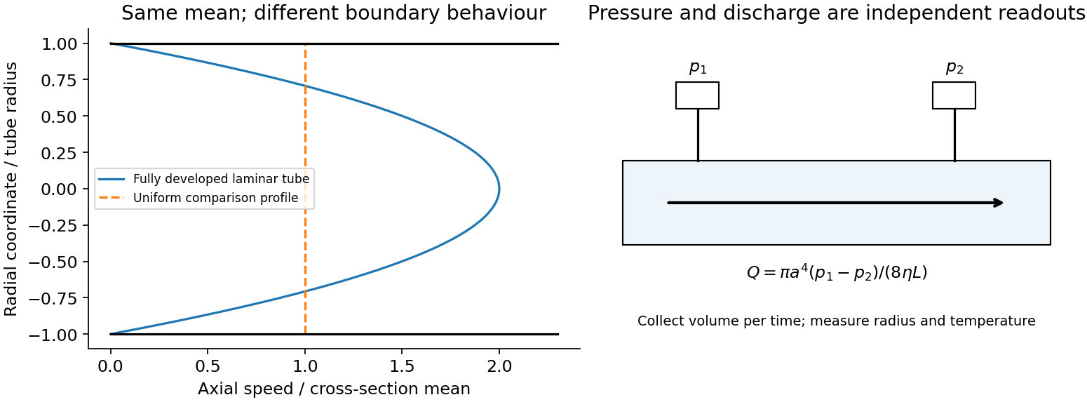
In a long straight circular tube, steady fully developed laminar flow hasThis Hagen-Poiseuille equation follows by balancing the axial pressure gradient with viscous shear and setting $v_z(a)=0$. The parabolic profile, the fourth-power radius sensitivity and the pumping power $\Delta pQ$ are experimentally distinct consequences. Entrance regions, rough walls, non-Newtonian response or a changing temperature require additional modelling.

The Reynolds number $\mathrm{Re}=\rho UL/\eta$ compares inertia with viscosity. Small values favor creeping-flow balances; high values permit thin boundary layers, separation and turbulence, although transition depends on geometry and perturbations, not one universal critical number. At high Reynolds number an outer flow can be approximately inviscid while near-wall viscosity still determines drag. This resolves why a zero-drag ideal potential-flow model cannot predict the resistance of an ordinary moving body. In turbulent flow, fluctuating Reynolds stresses redistribute momentum and increase the required pressure drop; averaging the equations introduces closure requirements.

A controlled tube experiment measures pressure difference and collected volume per time while changing forcing. Use tracers or a velocity probe to test profile shape, allow sufficient entrance length, and monitor radius and temperature independently. Repeat with reversed flow and at several rates to test offsets and linearity. Dye mixing alone does not measure viscosity or establish a fully developed velocity profile. The original figure below separates a specified laminar velocity profile from an independent pressure/discharge measurement.

A velocity field $\mathbf{u}(\mathbf{x},t)$ assigns a velocity to each point. Following a fluid parcel rather than holding position fixed gives the material or convective derivativeThe convective term can accelerate fluid even in a steady flow, for example as a stream narrows. Conservation of mass is ${\partial }_t\rho +\nabla \cdot (\rho \mathbf{u})=0$; constant-density incompressible flow has $\nabla \cdot \mathbf{u}=0$.

For an incompressible Newtonian fluid of constant density and viscosity, with conservative body-force potential per mass $\Phi$, momentum balance isNeglect viscosity and assume steady flow. Dotting with an element along a streamline, or using $(\mathbf{u}\cdot \nabla )\mathbf{u}=\nabla (u^2/2)-\mathbf{u}\times (\nabla \times \mathbf{u})$, givesThis is Bernoulli's equation: pressure work, kinetic energy and gravitational potential energy interconvert. In a connected irrotational region under the same assumptions, $B$ is the same for all streamlines. In a rotational flow it can vary between them. Viscous dissipation, pumps or unsteady motion require the corresponding modified balance; the steady inviscid expression cannot be applied indiscriminately.

Vorticity $\mathbf{\zeta }=\nabla \times \mathbf{u}$ measures local fluid rotation. For constant-density incompressible flow it evolves byshowing vortex stretching and viscous diffusion. A potential flow has $\mathbf{u}=\nabla \varphi$ locally, so irrotational incompressible motion satisfies ${\nabla }^2\varphi =0$. Boundary conditions then determine flows around simple shapes. A multiply connected region can have circulation even when its local vorticity vanishes; ideal potential flow also misses no-slip boundary layers and viscous drag.

For a Newtonian fluid, shear stress is proportional to strain rate. No-slip at solid walls produces velocity gradients and dissipation. Fully developed laminar pipe flow, for example, hasThe Reynolds number $\mathrm{Re}=UL/\nu$ compares inertial and viscous terms. Small values favour creeping-flow approximations; large values can permit thin boundary layers and turbulence, without guaranteeing turbulence in every geometry. The appropriate flow model follows from conservation laws, constitutive properties, boundaries and scale comparisons.

Viscosity transfers momentum between adjacent fluid layers. A Newtonian fluid has shear stress proportional to strain rate: for simple shear, $\boxed{{\tau }_{xy}=\eta \partial u_x/\partial y}$. Thus parallel plates of area $A$, separation $d$ and relative speed $U$ require force magnitude $\eta AU/d$ in a steady linear profile.

For an incompressible isotropic Newtonian fluid,for constant viscosity. With strain-rate tensor $e_{ij}$, the viscous dissipation rate per unit volume is $2\eta e_{ij}{e}_{ij}\ge 0$. Kinematic viscosity $\nu =\eta /\rho$ is the momentum diffusivity: a disturbance spreads over distance of order $\sqrt{\nu t}$.

The Reynolds number $\rho UL/\eta$ compares inertial and viscous forces. Small Reynolds number supports a creeping-flow approximation, while large values permit thin viscous boundary layers and possible turbulence. It does not mean molecular viscosity has disappeared. Gas viscosity results from molecular momentum transport; a liquid's microscopic transport depends strongly on intermolecular interactions. Non-Newtonian materials require a more general constitutive law.

Dynamic viscosity measures resistance to a velocity gradient. In Newtonian simple shear, ${\tau }_{xy}=\eta \partial u_x/\partial y$; positive viscosity dissipates mechanical energy into heat. Kinematic viscosity is $\nu =\eta /\rho$. For an incompressible fluid of constant viscosity,Scaling velocity by $U$ and length by $L$ gives the Reynolds number $\mathrm{Re}=\rho UL/\eta =UL/\nu$, the ratio of inertial to viscous terms. At small Reynolds number, creeping-flow approximations neglect inertia; at large Reynolds number, inertia dominates much of the bulk but viscosity can remain crucial in boundary layers. A large Reynolds number permits instability and turbulence; it does not by itself specify a universal transition threshold. Geometry and disturbances also matter.

A Newtonian fluid exerts viscous shear stress proportional to the rate of strain. For an incompressible fluid of constant dynamic viscosity $\eta$,The local momentum balance is the Navier-Stokes equation:The left side is density times material acceleration. A steady velocity field can still have convective acceleration when a moving parcel changes speed or direction; setting $\partial \mathbf{u}/\partial t=0$ does not eliminate it.

The Reynolds number $\mathrm{Re}=\rho UL/\eta$ compares inertia with viscous effects. At low Reynolds number, the fluid's own inertia can often be neglected, giving Stokes flow. This does not say that every immersed body has zero acceleration: its mass and the net pressure, viscous and body forces still enter its own equation of motion.

For a small rigid sphere moving through a slowly varying viscous background, Stokes drag is $-6\pi \eta a(\mathbf{v}-\mathbf{u})$. In still fluid, a simple settling model includes weight, buoyancy and drag:Ignoring fluid added mass and unsteady history forces, this gives relaxation time $m/(6\pi \eta a)$ and terminal velocityAt the terminal velocity the net force and acceleration vanish, while viscous drag and gravity remain individually nonzero. The dissipated power $6\pi \eta a{v}_t^2$ is supplied by the loss of gravitational potential energy relative to buoyant support. The creeping-flow and quasisteady-drag assumptions must be checked before applying this expression at large speed or immediately after a rapid start.

Following the moving fluid. The Eulerian velocity field $\mathbf{u}(\mathbf{x},t)$ assigns a velocity to each position. A fluid particle satisfies $\dot{\mathbf{x}}=\mathbf{u}$, so the chain rule gives the material derivative, also called the convective derivative,Even in steady flow a particle can accelerate because it moves between regions with different velocity. For example, flow around a curved obstacle changes direction despite ${\partial }_t\mathbf{u}=0$. Mass conservation isFor a constant-density incompressible fluid, $\nabla \cdot \mathbf{u}=0$.

Euler equations for an inviscid fluid and Bernoulli's equation. Neglect viscosity and take the body force per unit mass to be $-\nabla \Phi$. Newton's second law for a fluid element givesFor steady flow, dot with displacement along a streamline. The tangential component of $\mathbf{u}\cdot \nabla \mathbf{u}$ is the derivative of $u^2/2$ along that line. For constant density, integration givesIn uniform gravity, $\Phi =gz$. Thus pressure, kinetic energy per unit mass and gravitational potential energy per unit mass exchange along a streamline. For a barotropic compressible fluid, replace $p/\rho$ by $\int dp/\rho (p)$. Different streamlines need not have the same Bernoulli constant.

Vorticity and potential flow. Vorticity is $\mathbf{\omega }=\nabla \times \mathbf{u}$. A small fluid element rotates locally with angular velocity $\mathbf{\omega }/2$ after its deformational part is separated. The vector identitygives $\nabla B=\mathbf{u}\times \mathbf{\omega }$ for steady constant-density inviscid flow. Thus an irrotational region has one common Bernoulli constant on each connected region. In a simply connected irrotational domain, introduce a velocity potential $\mathbf{u}=\nabla \varphi$. Incompressibility then gives Laplace's equation, ${\nabla }^2\varphi =0$. For unsteady irrotational flow,An impermeable stationary wall fixes ${\partial }_n\varphi =0$, but ideal potential flow does not enforce no slip. In a multiply connected domain, irrotational flow may still have nonzero circulation around an excluded vortex core, so a globally single-valued potential requires care.

For example, uniform two-dimensional flow past a circular cylinder has $\varphi =U(r+a^2/r)\cos \theta$ outside $r=a$. Its normal velocity vanishes at the cylinder, and its surface tangential velocity is $-2U\sin \theta$. Bernoulli's equation predicts a symmetric pressure distribution and zero drag. This is D'Alembert's paradox: the assumptions omit the viscous boundary layers, separation and wake responsible for real drag.

For an incompressible fluid of constant kinematic viscosity $\nu$, the curl of the motion equation givesThe first term stretches and tilts vortex lines; the second diffuses vorticity. In two-dimensional incompressible inviscid flow the stretching term is absent and vorticity is carried with the fluid. In a three-dimensional inviscid flow it can be amplified by stretching. Density gradients not parallel to pressure gradients provide an additional source in a general compressible fluid.

Viscous flow. A Newtonian fluid's shear stress is proportional to rate of strain. For constant viscosity and incompressibility the Navier-Stokes equation iswith dynamic viscosity $\eta$ and kinematic viscosity $\nu =\eta /\rho$. At an ordinary solid wall, the no-slip boundary condition sets fluid velocity equal to the wall velocity. Viscosity transfers momentum between neighbouring layers and converts mechanical energy into heat; unlike the pressure force, its shear contribution depends on velocity gradients.

For plane Couette flow between plates $y=0,h$, with the upper plate moving at $U$, the steady solution is $u_x=Uy/h$, with shear stress $\eta U/h$. For pressure-driven flow through a pipe of radius $a$, a constant pressure gradient gives the parabolic Poiseuille profileThe Reynolds number $\mathrm{Re}=\rho UL/\eta$ compares convective inertia with viscous force. Small Reynolds number often permits the Stokes-flow approximation; large Reynolds number can produce thin boundary layers and, under suitable conditions, turbulence. It does not justify neglecting the wall conditions. Bernoulli's inviscid constant is generally not conserved along a viscous streamline, and pipe flow instead shows a pressure loss corresponding to dissipation.

The Magnus effect is the transverse force produced when a spinning body moves relative to a fluid. Rotation changes the flow and circulation around the body; the resulting asymmetric pressure and wake deflect the fluid, with the opposite transverse force on the body. Examples include the curved flight of spinning balls and the lift of rotating-cylinder sails.

A useful quantitative model is steady two-dimensional incompressible flow past a cylinder of radius $a$, with fluid velocity $\mathbf{U}=U\hat{\mathbf{x}}$ far away. Let circulation $\Gamma$ be positive anticlockwise as viewed from $+z$. The potential-flow velocity at the cylinder surface isThe Bernoulli equation outside the boundary layer givesIntegrating the pressure force around the cylinder, per unit span, yieldsThus the Kutta–Joukowski theorem givesThe sign here refers to the fluid velocity relative to the cylinder. For a body moving through otherwise stationary fluid, that relative fluid velocity points opposite to the body's translational velocity.

Real viscosity and the no-slip boundary condition transmit the surface rotation to the fluid and help set the circulation and separation pattern. Pure inviscid flow with only an impermeability condition does not determine $\Gamma$ from the cylinder's angular speed. Therefore the circulation must not be assigned a universal spin-rate formula without additional assumptions. The cylinder result illustrates the lift mechanism; quantitative forces on a finite spinning ball also depend on its geometry, Reynolds number, rotation rate, surface roughness and wake.

Use the pipe-diameter convention for the Reynolds number, with mean velocity $\bar{v}$, density $\rho$ and dynamic viscosity $\mu$:The Reynolds number compares inertial and viscous effects in the fluid flow. A conventional estimate for the onset of turbulence in a pipe is ${\mathrm{Re}}_{\mathrm{crit}}\simeq 2000$, givingHence the usual onset estimate is $\boxed{D\gtrsim 1.6\mathrm{mm}}$. Using the also common transition criterion ${\mathrm{Re}}_{\mathrm{crit}}=2300$ gives $1.84\mathrm{mm}$, whereas $\mathrm{Re}\gtrsim 4000$, used for established turbulence, gives $D\gtrsim 3.2\mathrm{mm}$. There is no universal sharp minimum: inlet disturbances and pipe conditions affect the transition from laminar flow, so the threshold convention must accompany the answer.

At a micrometre scale, viscous forces normally dominate inertia. As an illustrative Newtonian estimate, $L=1\mu \mathrm{m}$, $U=10\mu \mathrm{m}{\mathrm{s}}^{-1}$, $\rho =10^3\mathrm{kg}{\mathrm{m}}^{-3}$ and $\eta =10^{-3}\mathrm{Pa}\mathrm{s}$ give a Reynolds number $\rho UL/\eta =10^{-5}$. The surrounding flow is approximately a Stokes flow, satisfying $-\nabla p+\eta {\nabla }^2\mathbf{u}=0$ and $\nabla \cdot \mathbf{u}=0$.

A body of radius $0.5\mu \mathrm{m}$ translated at that speed in an unbounded Newtonian liquid would need Stokes drag $6\pi \eta aU\simeq 9.4\times 10^{-14}\mathrm{N}$. It stops almost immediately when propulsion stops. The scallop theorem rules out propulsion by a single reciprocal stroke in this ideal regime; a rotating helix or a nonreciprocal cycle of shapes can propel it. Brownian motion also randomizes position and orientation: Stokes–Einstein relation scales as $a^{-1}$ and rotational diffusion as $a^{-3}$, so retaining heading becomes harder as size decreases.

The Newtonian calculation is a scale estimate, not a complete model of blood. Vessel walls alter drag, the imposed flow advects the body, and nearby red blood cells make the medium heterogeneous at this scale. Non-Newtonian fluid effects and deformable obstacles can matter; steering must be assessed against those effects rather than inertial coasting.

For a microscopic swimmer, the Reynolds number $\mathrm{Re}=\rho UL/\eta$ is usually small. Taking $L=2\mu \mathrm{m}$, $U=20\mu \mathrm{m}{\mathrm{s}}^{-1}$ and water-like properties gives $\mathrm{Re}\simeq 4\times 10^{-5}$. The Stokes equations then balance viscous stress and pressure almost instantaneously, so a swimmer cannot coast appreciably when its propulsive stroke stops.

The scallop theorem rules out a reciprocal opening-and-closing stroke in an otherwise unchanged Newtonian environment: reversing the sequence of shapes reverses the motion, and changing the stroke speed does not prevent cancellation. Organisms therefore use nonreciprocal motion. A sperm-like bending wave travels along a flagellum; a bacterium can rotate a helical flagellar bundle. The unequal parallel and perpendicular drag of a slender filament converts those motions into a net thrust. A freely suspended swimmer is force-free and torque-free overall, so body drag balances thrust and the body counter-rotates against the rotating bundle. Tracking a body and its flagellum together can reveal these opposite rotations. The helical microswimmer with a spherical head makes that force and torque balance quantitative.

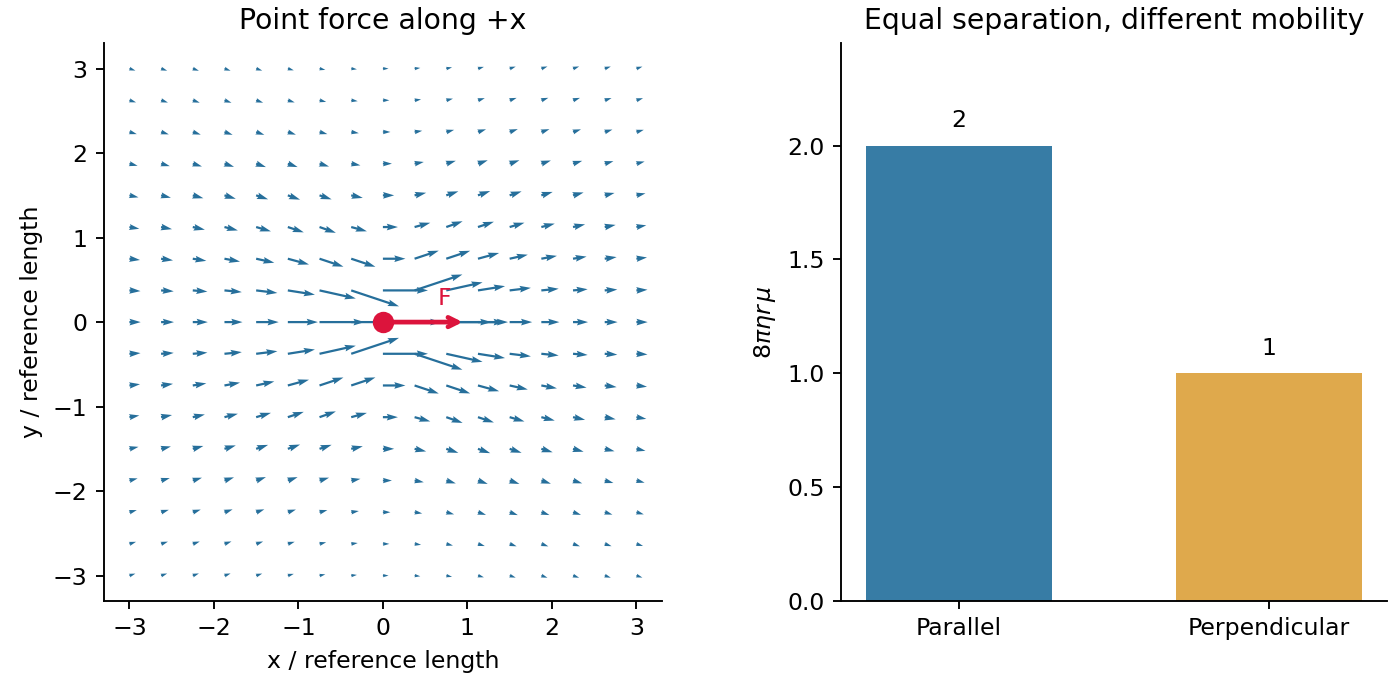
A moving or externally forced colloid disturbs the surrounding fluid, changing the velocity of other colloids even without direct contact. These hydrodynamic interactions are long-ranged at small Reynolds number. In an unbounded incompressible Newtonian liquid, the Stokes flow response to a point force is the Stokeslet:Its Oseen tensor isThis is a mobility tensor, with units velocity per force, rather than a stress tensor. At separation $r$ the response parallel to the line of centres is $1/(4\pi \eta r)$; the perpendicular response is $1/(8\pi \eta r)$. Flow is not isotropic even though the solvent is. The disturbance decays as $1/r$, so treating all drag forces as independent can miss correlated motion.

For well-separated equal spheres of radius $a$, the leading hydrodynamic mobility matrix givesThe first term is the isolated-sphere self mobility; the remaining terms couple distinct particles. At thermal equilibrium the fluctuation-dissipation theorem also predicts correlated short-time increments, $⟨\Delta r_{i\alpha }\Delta r_{j\beta }⟩\simeq 2k_{B}T{\mu }_{i\alpha ,j\beta }\Delta t$ with the configuration locally fixed. Thus correlated Brownian displacements can reveal hydrodynamic coupling without an applied force.

The point-force approximation requires $r\gg a$ and negligible inertia. It diverges at the origin and cannot replace the finite self mobility. Near-contact lubrication, walls, many-body corrections, and a viscoelastic solvent require more complete mobility laws. A force-free particle can instead have a faster-decaying leading disturbance, so the $1/r$ claim specifically concerns a net-force-driven object.