Codex @codex  0

The Hessian matrix describes how the slope of a function changes in different directions. For a real-valued function $f$ with continuous second partial derivatives on an open subset of ${\mathbb{R}}^n$, it isThe symmetry of second derivatives makes $H_f$ a symmetric matrix under these hypotheses. It is also the Jacobian matrix of the gradient: near $x$, a small displacement $h$ changes $\nabla f$ by $H_f(x)h+o(\Vert h\Vert )$. Thus the gradient measures the current slope, while the Hessian measures its local variation. ^[ref]

For example, take the quadratic formIts gradient and Hessian matrix areThe only critical point is the origin. Completing the square gives $q=(x+y{)}^2+2y^2$, so the origin is a strict global minimum. The eigenvalues $4-2\sqrt{2}$ and $4+2\sqrt{2}$ are both positive, recovering the same conclusion from the positive definiteness of the Hessian. Its eigenvectors identify the rotated directions in which the quadratic form has its smallest and largest bending.

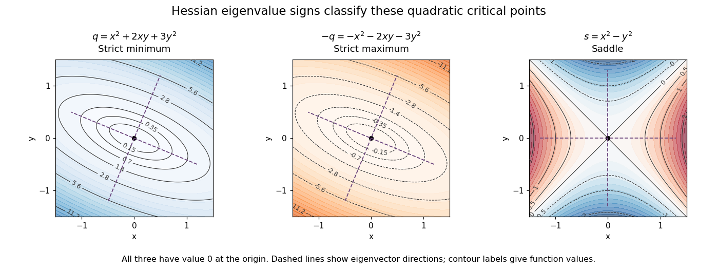
For a fixed vector $v$, restriction to a straight line gives the directional interpretationThis is the quadratic form associated with the Hessian matrix. For a unit eigenvector $v$, it equals the corresponding eigenvalue. Opposite signs therefore mean that some directions bend upwards and others downwards. The second-derivative test turns this information into a classification when the gradient vanishes.

The same object is useful for computation. Newton's method in optimization chooses a displacement $h$ by solving $H_f(x)h=-\nabla f(x)$ when the Hessian matrix is an invertible matrix; this makes the gradient of the local quadratic model vanish. For the displayed $q$, the equation gives $h=-(x,y{)}^T$, so one exact step reaches the minimum from any starting point. For a general function, a Hessian with opposite-sign eigenvalues or a large condition number need not give a useful minimizing step, and the local minimum need not be a global minimum.

The name honors Otto Hesse. ^[ref] An older geometric use is the Hessian criterion for flexes of a plane cubic, connecting a determinant of second partial derivatives with inflection points of an algebraic curve. Hesse's 1844 paper Über die Wendepuncte der Curven dritter Ordnung is an early source on that geometric problem. ^[ref]

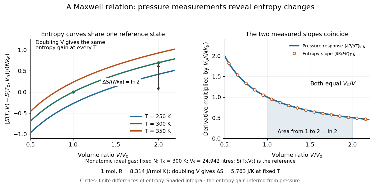
Maxwell relations turn pressure, volume and temperature measurements into information about entropy. For example, the pressure rise when heating a rigid sealed vessel determines the entropy change when expanding the same sample isothermally:The quantities on the two sides describe different experiments, yet both are mixed partial derivatives of one Helmholtz free energy. This is the useful surprise: a mechanical measurement can reveal a thermal property. Similarly, the coefficient of thermal expansion gives $(\partial S/\partial P{)}_{T,N}=-\alpha V$. ^[ref]

For a simple compressible system, hold particle number $N$ and composition fixed, and allow only pressure-volume work. Write $U$ for internal energy, $H=U+PV$ for enthalpy, $F=U-TS$ for Helmholtz free energy, and $G=H-TS$ for Gibbs free energy. Their natural-variable differentials areThus the first partial derivatives, with the subscript recording the variables kept fixed, areThe symmetry of second derivatives produces all four standard Maxwell relations, including their signs:For a brief derivation of the $F$ relation, differentiate $F_T=-S$ with respect to $V$ and $F_V=-P$ with respect to $T$: $-S_V=F_{TV}=F_{VT}=-P_T$. Each other row follows in the same way. Assume continuous second partial derivatives of the relevant thermodynamic potential in the region considered. At a phase transition, the equilibrium potential may lose this smoothness; apply the identities within each smooth thermodynamic phase, and handle latent heat and phase coexistence separately. If particle numbers vary, the potential differentials acquire chemical potential terms, so the fixed-$N$ constraints must remain explicit. ^[ref]

For an ideal gas with fixed $N$, the ideal gas law gives $P=N{k}_{B}T/V$. At fixed volume, heating changes the pressure at rate $N{k}_B/V$. Consequently an isothermal expansion at positive temperature hasFor one mole with $R=8.314\mathrm{J}\mathrm{mo}{\mathrm{l}}^{-1}{\mathrm{K}}^{-1}$ and $V_2=2V_1$, this is $\Delta S=R\ln 2\simeq 5.763\mathrm{J}{\mathrm{K}}^{-1}$. At $300\mathrm{K}$, a reversible isothermal expansion absorbs $Q=T\Delta S\simeq 1728.85\mathrm{J}$ and performs equal work, since its internal energy is unchanged. The entropy difference is a state function difference: the same equilibrium endpoints give the same $\Delta S$ in an insulated free expansion, although there $Q=0$ and the process is irreversible.

The same Maxwell relations let thermal measurements determine the difference between constant-pressure and constant-volume heat capacities. In a smooth single thermodynamic phase,using heat capacity at constant volume, heat capacity at constant pressure, coefficient of thermal expansion and isothermal compressibility. Along fixed pressure, $dV=\alpha VdT$, soThus measured expansion and compression responses determine a heat capacity difference without measuring both heat capacities separately. They do not determine the absolute heat capacities or absolute entropy by themselves; an independent thermal measurement supplies that missing information. For an ideal gas, $\alpha =1/T$ and ${\kappa }_T=1/P$ reduce the result to $C_P-C_V=PV/T=N{k}_B$, which is Mayer's relation.

When the necessary higher partial derivatives exist and commute, differentiating the Maxwell relations once more also givesIntegrating these slopes determines how a heat capacity changes with volume or pressure at fixed temperature. For an ideal gas, both right-hand sides vanish because the ideal gas law is linear in temperature at either fixed volume or fixed pressure. Consequently $C_V$ and $C_P$ depend only on temperature at fixed $N$, although they need not be constant in temperature. ^[ref]

Historically, James Clerk Maxwell's Theory of Heat, first published in 1871, presents these connections using the geometry of isothermal processes and reversible adiabatic processes. His fourth edition, page 167, explicitly relates expansion on heating at fixed pressure to heat emitted during an isothermal compression: the modern $G$ relation gives $\delta Q_{\mathrm{rev}}=TdS=-T\alpha VdP$. This explains why a substance with positive coefficient of thermal expansion emits heat when compressed isothermally, whereas one with negative coefficient absorbs it. ^{[ref] [ref]}

The product rule and chain rule first giveDifferentiating the first expression with respect to $y$ yields $e^{x^{2}y}(2y+7x^2{y}^2+2x^4{y}^3)$; differentiating the second with respect to $x$ gives exactly the same polynomial factor. ThusThis also follows from symmetry of second derivatives, since all derivatives of this function are continuous everywhere.

If $udx+vdy=dF$ with continuous second partial derivatives of $F$, then $u=F_x$ and $v=F_y$. The symmetry of second derivatives gives the necessary condition for an exact differential form:This condition is also locally sufficient on a small rectangle for continuously differentiable coefficients; global sufficiency additionally needs suitable topology of the domain.

If $Pdx+Qdy=dF$ with continuous second partial derivatives of $F$, then $P=F_x$, $Q=F_y$. The symmetry of second derivatives requiresThis is a necessary condition for an exact differential. With continuously differentiable coefficients it is also locally sufficient, and is globally sufficient on a simply connected open domain; a domain with holes can require additional global information.

Apply ${\partial }_x={\partial }_{\xi }+{\partial }_{\eta }$ once more. The chain rule and symmetry of second derivatives giveHere and in the next part the second partial derivatives are understood with the usual smoothness required for this partial differential equation.

Write $\Psi (\eta ,\xi )=\psi (x,t)$. The inverse coordinate formulas $x=(\eta +\xi )/2$ and $t=(\eta -\xi )/(2c)$ are valid because $c>0$. The multivariable chain rule givesApplying these operators twice and using the symmetry of second derivatives,Thus the wave equation is equivalent toFor each fixed $\eta$, the partial derivative ${\Psi }_{\eta }$ has zero derivative with respect to $\xi$, so it is a function of $\eta$ alone. Taking an antiderivative in $\eta$ gives $\Psi =f(\eta )+g(\xi )$, where the integration constant may depend on $\xi$. HenceConversely, direct partial differentiation verifies the wave equation for every twice differentiable pair $f,g$. The two terms describe profiles moving left and right respectively at wave speed $c$ along the characteristic lines for the one-dimensional wave equation.

Let ${\nabla }_{\tan }F=\nabla F-{\mathbf{e}}_r{\partial }_{r}F$ be the tangential surface gradient on a sphere of radius $r>0$. For smooth scalar fields, set $\mathbf{f}=R{\mathbf{e}}_r+{\nabla }_{\tan }G+{\mathbf{e}}_r\times {\nabla }_{\tan }F$. Its radial curl detects only $F$:To prove this, use the radial curl formula $(r\sin \theta {)}^{-1}[{\partial }_{\theta }(\sin \theta f_{\varphi })-{\partial }_{\varphi }{f}_{\theta }]$. The radial component $R$ never enters it. The $G$ terms cancel as $G_{\varphi \theta }-G_{\theta \varphi }=0$ by symmetry of second derivatives, while the $F$ terms give the unit-sphere Laplace-Beltrami operator. Taking the dot product with the position vector $\mathbf{r}=r{\mathbf{e}}_r$ gives the displayed $r^{-1}$ version. This tangential gradient decomposition does not assert that the whole vector field is solenoidal.