Topics (384k) Articles (398k) Users (410) Discussions (242) Comments (383) Files (13k) New article

Geological Society of America Bulletin 60, 1837–1856.
A gear inspection missing-area bound limits the whole-target pitting fraction using the area actually observed and explicit constraints on the unseen area. It formalizes what a gear inspection coverage audit can establish without assuming that excluded regions resemble visible ones.
Let , let be the observed gear pitting area fraction, and let be the unseen fraction affected by pitting. For a consistent surface-area convention,With only known,The interval width is exactly . Improving classification precision within the visible area cannot by itself remove uncertainty from a completely unseen region.
For an original example with and , the possible whole-target fraction ranges from to . The observed therefore does not prove that the whole surface is below an illustrative criterion. That chosen criterion is not a gear safety or acceptance standard.
The worst-case upper bound meets a target only iffor . At and , at least about coverage is required for this particular worst-case guarantee.
Additional justified information can narrow the range. If a separate observation establishes , then . At and , this gives . The tighter bound depends on the new evidence about the unseen region, not on a mathematical preference for a smaller interval.
These deterministic bounds assume the observed classification and represented areas are correct. Image registration, image segmentation and geometric uncertainties can require additional allowances. They are not confidence intervals and do not describe pit depth or remaining fatigue life. The primary NASA endurance study combined inspection with vibration and debris monitoring; these different observations constrain different aspects of damage.[ref]
Gear Fault Detection Effectiveness as Applied to Tooth Surface Pitting Fatigue Damage by David G. Lewicki and others. Printed pp. 2–5, inspection and monitoring comparisons
Gear tooth load sharing is the division of transmitted mesh load among simultaneously contacting tooth pairs. Gear contact ratio determines how engagement intervals overlap, but it does not by itself specify each pair's force. Tooth and support deformation, profile geometry and operating speed affect that distribution. A primary dynamic analysis explicitly coupled tooth stiffness with calculated dynamic loads rather than assigning a fixed full load to every active pair.[ref]
An illuminating quasistatic model treats active pairs as parallel springs with a common normal approach . With pair stiffnesses and no gaps, , soThe stiffness sum is gear mesh stiffness, and is a gear tooth load fraction. If two active pairs have stiffness100 and150N/µm under total normal load1000N, their common approach is4µm and loads are400 and600N. Equal sharing requires equal effective stiffness in this particular model.
Include a geometric gap by writing . If the second pair has a2µm gap, the same1000N total load gives with measured in micrometres. The result is , and . At only100N, the first pair alone compresses1µm, leaving the second pair out of contact.
For an ideal spur gear mesh with transverse contact ratio between1 and2, the fraction of a tooth-entry cycle having two pairs in contact is . A ratio1.635 therefore gives about63.5% two-pair contact and36.5% single-pair contact. This is geometric timing, not a guarantee of equal forces in the overlapping part. A gear friction work per engagement calculation must use each pair's own load history; dynamic motion can require more than the quasistatic spring approximation.
Consider the explicitly specified objectiveand estimate its derivative by a symmetric finite difference with step . The choice of shared or independent noise changes the estimator's variance even though both use correct normal distributions at the two parameter values.
With common random numbers, the same appears on both sides:Thus and , independent of . Cancellation removes the noisy square term. For this quadratic, the symmetric difference has no truncation bias in exact arithmetic.
For independent standard normals , instead useIf , expand . The standard-normal moments , and giveAdding the two independent square variances and dividing by yieldsBoth estimators have the correct expected value , but the independent-noise variance diverges as tends to zero. At and , the variances are and . An average of independent replicate estimators divides each variance by .
This is a complete calculation for the stated quadratic, not a universal dominance theorem. At , and , the independent variance is , below the shared value . The covariance principle in common random numbers explains why coupling needs a specified objective and comparison. Very small steps in floating-point evaluation also introduce cancellation concerns that this exact-arithmetic model does not include.
Quadratic energy loss from centred Gaussian gate timing error is the leading decrease in collected energy when a symmetric gate is displaced slightly from the centre of a Gaussian pulse. At the optimum the first-order change vanishes, but the second-order change is negative. The Gaussian pulse time-gate energy fraction gives the exact displaced-gate integral; here the local loss and its effect on jitter are derived explicitly.
Let be the centred energy-normalized pulse profile, let , and setThe Leibniz integral rule gives . Since is even and ,The Taylor expansion therefore yieldsThis is an absolute fraction of the full pulse energy. The relative loss compared with the centred gate is instead .
For a gate as wide as the power FWHM , and . An offset gives leading loss , or about percent of the centred gate's collected energy. Neither the full pulse energy nor the gate width has changed.
A zero mean offset does not eliminate this loss. For a sufficiently narrow random offset with mean and variance , the leading expectation isIf has a centred normal distribution, the quadratic model also gives . At , the leading mean loss is and this standard deviation is . These formulas neglect fourth-order effects; they are local approximations, not bounds for large timing excursions.
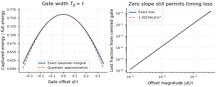
Exact Gaussian gate capture and its local quadratic loss: a zero first derivative does not remove timing sensitivity.
Details. An apparatus check scans the gate delay about its optimum and compares the measured decrease with the model, while monitoring gate width and the pulse. A gate on the detector's electrical output need not act directly on optical power: the detector impulse response and readout convolution must be included. NIST's impulse-response measurements illustrate that distinction.[ref]
A special function of bounded variation is a function of bounded variation on a domain whose distributional derivative has no diffuse singular part. Writing the derivative measure as an absolutely continuous part, a jump part and a remaining Cantor part,the defining condition is . The space is denoted . Here is the jump set and are the two traces across it; and are Lebesgue measure and Hausdorff measure.
On an interval containing zero, has derivative a Dirac measure at zero and belongs to : jumps are allowed. The Cantor function instead has a diffuse singular derivative and is not in . Thus “special” separates sharp interfaces from more distributed singular variation. This makes useful for image segmentation and variational models with both bulk and interface energies.[ref]
A floating-pinion contact-loss check tests whether the motion predicted by a floating-pinion balancing mode remains compatible with every contact assumed to be compressed. It prevents a two-contact linear solution from being extrapolated into tensile tooth forces.
For the symmetric modelwith , mismatch , displacement and fixed mean approach , both contacts are compressed only whenAt equality one modeled force is zero. Outside the interval the linear expression makes one force negative; the unilateral model must replace that value by zero and the force-balance equations must be solved again.
Write and define the floating-pinion compression marginIf the motion satisfies , then is sufficient to retain both contacts. For a steady single sinusoid of amplitude and fixed , the maximum of over a complete cycle is , making the condition exact for that stipulated motion.
An original example uses , and . The margin is . A sinusoidal amplitude retains a minimum compression ; with , the smallest contact force is . Amplitude instead makes the unconstrained formula reach , revealing a contact-loss inconsistency rather than a physical tensile contact.
For a damped transient, an amplitude envelope is a sufficient bound but need not be attained at the phase where contact is least compressed. Failure of that sufficient envelope test therefore calls for examining the actual trajectory; it is not automatically proof that a real contact opened.
A controlled dynamic test can compare displacement with load-sensitive observations and check whether the assumed contact set persists. The historical face-gear program examined mounting freedom and torque division under slow rolling; it did not validate every possible dynamic contact assumption.[ref]
Development of Face Gear Technology for Industrial and Aerospace Power Transmission by Gregory F. Heath and others. Introduction, printed pp. 1–2; Conclusions, printed p. 84, floating versus constrained mounting
Early-time resistance dominance of a filling response means that the initial volume admitted by a pressure step is governed mainly by airway resistance, even when the eventual volume depends strongly on lung compliance. For a passive compartment with constant airway resistance , lung compliance , imposed pressure increment and initial added volume zero,Initially the elastic recoil increment is zero, so the initial volumetric flow rate is . The initial slope identifies within this model, not .
A Taylor series makes the separation explicit:Information about lung compliance first enters the curvature. Recovering that curvature from noisy early measurements can be much harder than measuring the initial slope. The dimensionless ratio controls the approximation: the exact response divided by the resistance-only prediction is .
For an original calculation, take , and compare with . Both predict initial volumetric flow rate 1 L/s. At 0.05 s their admitted volumes are approximately 0.04877 and 0.04975 L, although their equilibrium added volumes are 1 and 5 L. An apparently precise short filling trace can therefore provide little discrimination between very different equilibrium lung compliances.
This is an ideal pressure-step calculation. A finite instrument response, an unknown driving pressure, nonlinear airway resistance or multiple compartments changes what can be inferred. A primary ventilation study explicitly measured multiple expiratory time constants because deflation need not follow one exponential.[ref]
Static and Dynamic Measurements of Compliance and Driving Pressure: A Pilot Study by Pierre Tawfik and others. Materials and Methods, Study Procedures: two expiratory time constants rather than an assumption of uniexponential deflation
An early filling slope and an equilibrium lung compliance answer different experimental questions.The layer-thickness tradeoff in erosion-density sampling balances spatial averaging bias against uncertainty in the small mass and volume of a sampled surface layer. A thinner layer can better represent boundary density while being harder to measure precisely. The preferred thickness depends on the measurement model and the required inference, rather than being a material constant.
In an original locally planar model, layer density is estimated as , with area and thickness . For boundary density and outward density gradient , finite-shell bias in boundary-density calibration gives leading bias . Suppose the standard uncertainties and are independent and approximately constant over the tested thickness range. First-order propagation givesThe final term assumes independent area uncertainty; correlations require additional terms. The GUM supplies the general correlated-input propagation rule.[ref]
Write and . The resulting squared-error planning objective isFor nonzero , differentiation gives . The area term raises the error floor in this approximation without changing the optimum; thickness uncertainty changes the optimum through .
For stipulated , , and g, neglecting thickness uncertainty gives mm. Including cm, or 1 micrometre, gives and mm. These are original planning examples, not prescribed section thicknesses.
Thickness-uncertainty limit in erosion-density sampling becomes important when small layers approach the dimensional readout's resolution. If the feasible interval excludes the calculated optimum, optimize over the actual interval and test whether the local-gradient and planar approximations remain adequate. If , this simplified model has no finite interior optimum; other constraints determine the usable thickness.
A proposed experiment uses matched conditioning, several layer thicknesses and recorded mass-difference correlations. Sectioning damage or density changes during drying can invalidate the assumed error model. Kureha's polyglycolic acid experiment measures filtered, dried retained solids after water exposure.[ref] Local density sampling is an additional measurement, and its tradeoff should be assessed separately from the retained-mass curve.
The transit radius is the effective radius inferred from the fraction of stellar radiative flux blocked during an exoplanet transit. For a uniformly bright star, a completely overlapping opaque planet gives transit depth . Thus a one-percent depth corresponds to a radius ratio of about one tenth.
Real inference accounts for limb darkening, transit geometry and contaminating light. A planetary atmosphere can make the effective occulting area depend on wavelength: a grazing ray traverses a long slant path, so absorption need not correspond to one sharply defined material surface. A quoted transit radius therefore belongs to a measurement band and a stated model.[ref]
Analytic Light Curves for Planetary Transit Searches by Kaisey Mandel and Eric Agol. Sections 2, 4 and 5, geometry, limb darkening and small-planet approximation
An etalon coating group delay is the frequency derivative of the reflection phase contributed by the two coatings during one internal round trip. At fixed incidence and polarization, write the internal reflection coefficients as . With the phase convention of etalon round-trip phase,The phases must refer to consistently chosen surfaces: moving a reference plane transfers a propagation contribution between the terms. Only the consistently defined total is directly comparable with the resonance spacing.
A constant coating phase changes the positions of resonances but contributes zero group delay. A linear phase produces constant group delay. Curvature produces group delay dispersion:A highly reflecting coating therefore cannot be characterized by reflectance alone. The manufacturer's ultrafast-mirror documentation separately specifies reflection dispersion and shows multiple-bounce arrangements for compensation.[ref]
Chirped Mirrors by Thorlabs. Dispersion-Compensating Mirrors, phase/GD/GDD characterization and Fig. 1.1
For an original constant-slope example, suppose propagation contributes and the coatings together contribute . The local free spectral range is approximately , rather than . Ignoring coating delay would overassign that to propagation when inferring a spacer thickness or group index. The values are stipulated, not a coating specification.
For an independent curvature example, let the summed coating phase contain , with . Across a frequency interval , its group delay changes by . The derivative is with respect to angular frequency; omitting changes the result.
Experimentally, one may measure adjacent resonance frequencies and compare their spacing with an independently characterized spacer and group index. A discrepancy alone cannot uniquely identify coating delay: spacer dispersion, incidence angle and geometry also affect the result. Etalon delay inferred from free spectral range gives an interval-averaged phase slope; identifying it with a single-frequency derivative requires sufficiently slow variation. The simple manufacturer's spacer relation explicitly neglects spacer dispersion.[ref]
Etalon Tutorial by Iridian Spectral Technologies. Free Spectral Range section and displayed plate relation
A higher-harmonic penalty in span loading is the increase of ideal lift-induced drag caused by nonfundamental terms in a wing's circulation distribution at fixed total lift and span. In the classical planar lifting-line theory expansion, choose andHere is span, is freestream speed, and the coefficients are dimensionless. The primary force calculation uses this circulation expansion, the local lift law and sine orthogonality to obtain the lift and induced drag.[ref]
Force Calculations for Lifting Line (16.100) by MIT OpenCourseWare. printed pp. 1–3, circulation expansion and force integration
Because and , the integral for total lift selects only . The induced angle contains . Integrating its product with the loading then givesThe orthogonality identity behind both reductions isA higher harmonic can thus have zero net lift contribution while still adding positive induced drag. Its effect on local loading has not disappeared merely because its span integral vanishes.
For nonzero , division by the elliptic reference givesThe pure first harmonic gives elliptic span loading and . At a fixed relative coefficient magnitude, a larger order carries a larger penalty. Changing a coefficient's sign can redistribute the loading without changing its own squared contribution in this ideal model.
For an original example, take , and all other higher terms zero. The excess is , so . With and ,At and , the corresponding induced drags are about and . The higher harmonics add to this induced contribution, rather than to every source of aircraft drag.
A truncation error in an inferred span-efficiency factor matters when fitting sparse load measurements. Omitting nonzero terms makes the ideal-model drag sum too small at a fixed known , while fitting noisy high orders can inflate it because the terms are squared and weighted by order. If a justified bound is , then . A fit residual alone does not supply that bound.
A proposed experiment reconstructs section lift or circulation from a spanwise pressure survey, fits a declared set of modes, and compares the predicted induced contribution with an independent wake-based estimate. Report sampling density, load uncertainty and truncation choice. Viscosity, compressibility, nonplanar geometry or constraints other than fixed lift and span change the physical optimization problem; the quadratic penalty belongs to the stated lifting-line model.
The proximal isovelocity surface area method estimates instantaneous flow towards a leaking heart valve from the upstream convergence field. Color Doppler supplies a contour at a chosen aliasing speed . If that contour represents a hemisphere of radius , flow approximately normal to it giveswhere the matched jet speed comes from continuous-wave Doppler echocardiography. The inferred effective regurgitant orifice area is a flow-equivalent area, not the area of the colored region or necessarily the anatomical hole.[ref]
The physical idea is conservation of mass. More generally, . Replacing that integral by one speed times a surface area requires an appropriate velocity component and geometry. Doppler ultrasound measures a component along the beam, so an apparent constant-color contour is not automatically a measured three-dimensional surface of constant normal speed.
For an original hemispherical example, let cm and cm/s. The modeled backward flow is mL/s. With matched cm/s, the effective area is . If this area remains constant and the velocity-time integral is 140 cm, the modeled regurgitant volume is 25.33 mL. These are stipulated inputs, not severity thresholds.
Geometry and timing can each change that inference. In an ideal radial model restricted to a known solid angle , ; a hemisphere uses . Thus a stipulated gives half the flow at the same radius and speed. This illustrates flow-convergence angle correction; a real nonhemispherical or confined flow needs a justified geometric model rather than an arbitrary numerical adjustment.
Likewise, a radius observed at one instant must be paired with the jet speed at that instant. A peak effective area multiplied by a full-cycle velocity integral can overstate transported volume when the leak occupies only part of systole. The technical report explicitly discusses matching times, nonplanar convergence and changing regurgitant duration.[ref]
Recommendations for Noninvasive Evaluation of Native Valvular Regurgitation by William A. Zoghbi and others. Section II.B.6.c, pp. 312–313, timing, duration and shape qualifications
The apparatus observes an aliased velocity pattern and a jet spectrum; the flow and area are derived through the stated model.Coupled normal-contact penalty modes are small oscillations generated by several simultaneously compressed penalty contacts acting through shared body inertia. A displacement at one contact can accelerate another because both load the same translating or rotating bodies. Separate scalar effective mass in a normal-contact penalty mode estimates do not generally give the coupled frequencies.
Freeze a contact configuration, use independent generalized displacement perturbations , positive-definite mass matrix , and gap perturbations . Let be a positive diagonal matrix of normal penalty stiffnesses. After subtracting equilibrium loads, the restoring generalized force is , soThe contact-Jacobian force/velocity pairing and stiff compliant-contact model come from the primary multibody formulation; the local modal reduction here follows by substitution.[ref]
Although need not be symmetric, it is similar to the symmetric positive-semidefinite matrix . Set to obtainIts positive eigenvalues are squared angular frequencies. A zero eigenvalue may describe redundant gap coordinates outside the realizable displacement subspace; it should not automatically be interpreted as an extra physical oscillation. Free generalized motions satisfying are a separate possibility.
For an original planar example, a rigid bar has vertical translation , small rotation , mass , center-of-mass moment of inertia , and two vertical contacts at horizontal offsets . ThenWith equal contact stiffness , the equal-gap mode is vertical translation and the opposite-gap mode is rocking. Their angular frequencies areTake , , and . Then has diagonal entries and off-diagonal entries . Its eigenvalues are and , giving and . Treating the contacts independently would assign each and miss the faster rocking mode.
Contact-mode timestep stability depends on the largest active frequency and on the integrator. For the undamped central-difference recurrence, one mode has amplification equationThe distinct oscillatory roots lie on the unit circle for ; the endpoints need separate treatment. The example therefore requires for this linear stability condition. Resolving the waveform accurately normally requires a smaller step. This is not a stability rule for every integration method.
The derivation applies while both contacts remain compressed and geometry is locally constant. A sufficiently large rocking amplitude can unload one contact, changing the active model. A proposed check preloads both supports, applies small symmetric and antisymmetric perturbations, and compares measured or simulated frequencies with the two predictions. Repeat with smaller amplitudes and smaller timesteps to separate linearization error, contact opening and numerical error.
Homogeneity-study time-term identifiability asks whether a measurement schedule supplies enough independent information to distinguish instrumental drift from differences between containers. Adding time to a regression analysis does not guarantee that its coefficient can be estimated separately from the container effects.
In an original fixed-container measurement model,each container has an unknown intercept and all share a linear drift rate . If every observation of container occurs at one time , any rate gives the same predictions after replacing by . The data cannot distinguish those parameter sets. Algebraically, the time column lies in the span of the container-indicator columns of the design matrix.
Repeated observations at different times within at least one container can break that exact ambiguity. Subtract each container's mean:For independent, equal-variance errors with variance , the least-squares drift estimate hasprovided the denominator is positive. The formula distinguishes identifiability from precision: a positive but tiny within-container time spread permits a formally unique yet noisy estimate.
For three containers each observed twice one time unit apart, the denominator is . If each pair is instead separated by five time units, it is . With the same residual variance and a valid linear-drift model, the latter schedule reduces drift-estimate variance by 25, or its standard deviation by five. These are design calculations, not a guarantee that a longer experiment remains linear or stable.
Randomized order and controls address additional risks. The primary IUPAC protocol requires randomized analysis of duplicate portions and inspection for suspect data features.[ref]
The International Harmonized Protocol for the proficiency testing of analytical chemistry laboratories by Michael Thompson and others. Appendix 1, A1.1 and A1.3
NIST's comparison designs also use observation order to suppress specified drift contributions.[ref]Record timestamps and check the rank of a matrix for the fitted design, but also assess residual time patterns, uncertainty and physical plausibility. A randomized schedule can still have poor numerical leverage; a full-rank model can still be wrong. Drift-aware homogeneity analysis must report those distinctions rather than equating a returned regression coefficient with established material homogeneity.
A velocity-weighted Doppler profile correction converts an integrated sampled velocity into an integrated area-mean velocity by weighting each instantaneous correction according to the sampled velocity at that time. For a fixed opening of cross-sectional area , suppose its area-mean normal velocity is . Thenprovided the denominator is nonzero. Applying the time average of to a velocity-time integral generally answers a different question.
The error has an exact covariance form. Define and time covariance . ThenConsequently an unweighted correction is exact if that covariance vanishes, even when the correction varies in time. Its failure is about how profile changes align with transport, not merely whether either trace varies.
In an original two-second example, equal one-second intervals have sampled velocities 10 and 40 cm/s and corrections 1.0 and 0.5. The unweighted mean correction is 0.75, but . With , actual modeled transport is 60 mL; unweighted correction predicts 75 mL, a 25% overestimate. Here time covariance is cm/s and mean sampled velocity is 25 cm/s, recovering .
If is nonnegative, normalized velocity weights are nonnegative and lies between the instantaneous corrections. For reversing fluid flow, the denominator can instead approach zero through cancellation. Forward and reverse transported volumes can then be more informative than a single unstable ratio. If opening area changes, the integral must also retain ; this fixed-area correction does not remove that additional dependence.
The primary Doppler report requires appropriate matching of sampled velocity and anatomical area and distinguishes modal spectral velocities from the fastest envelope.[ref]
Recommendations for Quantification of Doppler Echocardiography by Miguel A. Quiñones and others. PW Doppler and CW Doppler, printed pp. 168–169
The covariance calculation is an original integration identity, not a universal clinical profile correction.The first angular moment of a radiance field is the vectorwith units for frequency-integrated radiance. It records a directional imbalance. Here is the viewing direction toward the arriving light, as in dipole anisotropy of a radiance field; using propagation directions instead reverses the vector. With that convention change, this is the bolometric vector form of the radiative flux, an existing radiation-field moment.
Opposite ideal planar receivers measure this moment without assuming a pure dipole. Since , the cosine-response irradiance formula givesThree orthogonal receiver pairs therefore determine the three components. For original differences , the moment has those components and magnitude . The derivation requires the same spatial field, stable gains and known angular response. The primary optical guide describes cosine-receptor characterization rather than assuming it perfect.[ref]
A zero first moment does not establish an isotropic radiance field. For example, two equal oppositely directed collimated beams have cancelling vector moments while remaining strongly directional. Conversely, any nonzero first moment rules out isotropy. The scalar all-direction integral bounds the moment by for nonnegative radiance, by the triangle inequality and .
The knife wedge angle is the included angle between the blade faces meeting at a cutting edge. It is a property of the edge geometry, distinct from the knife clearance angle produced by orienting the knife relative to the specimen. A final bevel can have a different angle from the broader blade body, so identify which faces define a quoted angle.[ref]
Knife Angle in Microtomy by Charles W. Scouten. Ideal versus compromise: final bevel and cross-sectional wedge
In ultramicrotomy, the wedge angle affects the tradeoff between reducing section compression and supporting a durable edge. Manufacturer descriptions distinguish and diamond knives; the lower-angle family is described as reducing compression. Guidance for polymer and brittle-material sectioning also emphasizes that lower angles leave a more sensitive edge and that some hard materials favor a larger angle.[ref]
Ultra diamond knives by DiATOME. ultra35° and ultra45° descriptions
[ref]Ultramicrotomy Techniques for Materials Sectioning by Leica Microsystems. How to prepare high-quality sections of polymers; brittle-material discussion
An original geometric comparison makes the difference concrete without pretending to predict cutting forces. On each face of an ideal wedge, mark a point a distance from the apex. The distance between those points is the base of an isosceles triangle:For , this gives at and at . The larger angle puts more material between the faces at that distance from the apex. This geometry is not an empirical law relating wedge angle to force, friction or a particular compression percentage.
Changing knife clearance angle rotates both blade faces together and leaves their included angle unchanged. Conversely, selecting a different wedge geometry need not mean that the same holder setting gives the same cutting conditions. A meaningful comparison records both angles, specimen material, feed and observed section compression. The two angle names should therefore remain separate even when an instrument discussion informally calls either one the knife angle.
Pinned article: Introduction to the OurBigBook Project
Welcome to the OurBigBook Project! Our goal is to create the perfect publishing platform for STEM subjects, and get university-level students to write the best free STEM tutorials ever.
Everyone is welcome to create an account and play with the site: ourbigbook.com/go/register. We belive that students themselves can write amazing tutorials, but teachers are welcome too. You can write about anything you want, it doesn't have to be STEM or even educational. Silly test content is very welcome and you won't be penalized in any way. Just keep it legal!
Intro to OurBigBook
. Source. We have two killer features:
- topics: topics group articles by different users with the same title, e.g. here is the topic for the "Fundamental Theorem of Calculus" ourbigbook.com/go/topic/fundamental-theorem-of-calculusArticles of different users are sorted by upvote within each article page. This feature is a bit like:
- a Wikipedia where each user can have their own version of each article
- a Q&A website like Stack Overflow, where multiple people can give their views on a given topic, and the best ones are sorted by upvote. Except you don't need to wait for someone to ask first, and any topic goes, no matter how narrow or broad
This feature makes it possible for readers to find better explanations of any topic created by other writers. And it allows writers to create an explanation in a place that readers might actually find it.
Figure 1. Screenshot of the "Derivative" topic page. View it live at: ourbigbook.com/go/topic/derivativeVideo 2. OurBigBook Web topics demo. Source. - local editing: you can store all your personal knowledge base content locally in a plaintext markup format that can be edited locally and published either:This way you can be sure that even if OurBigBook.com were to go down one day (which we have no plans to do as it is quite cheap to host!), your content will still be perfectly readable as a static site.
- to OurBigBook.com to get awesome multi-user features like topics and likes
- as HTML files to a static website, which you can host yourself for free on many external providers like GitHub Pages, and remain in full control

Figure 2. You can publish local OurBigBook lightweight markup files to either OurBigBook.com or as a static website.
Figure 3. Visual Studio Code extension installation.
Figure 5. . You can also edit articles on the Web editor without installing anything locally. Video 3. Edit locally and publish demo. Source. This shows editing OurBigBook Markup and publishing it using the Visual Studio Code extension. 
- Infinitely deep tables of contents:



All our software is open source and hosted at: github.com/ourbigbook/ourbigbook
Further documentation can be found at: docs.ourbigbook.com
Feel free to reach our to us for any help or suggestions: docs.ourbigbook.com/#contact