Topics (384k) Articles (398k) Users (410) Discussions (242) Comments (383) Files (13k) New article
A reference-junction temperature sweep tests a thermocouple measurement system by varying its connection-region temperature while holding the thermocouple measuring junction at an independently known, stable temperature. The intended invariant is the inferred measuring-junction temperature after cold-junction compensation; the raw electric potential difference is expected to change.
Let be the thermocouple reference function, the fixed measuring-junction temperature, the actual terminal temperature and the reference-sensor reading. In an ideal matched readout,If , the sum inside the inverse function stays equal to throughout the sweep. This tests the thermal reference and the compensation calculation together; it does not require the raw signal to be constant.
A primary design verification by Mike Beckman and Luis Chioye places the ADS1118 board and reference connections in a temperature-controlled environment, while the other end of the thermocouple remains in a stable bath. Its Figure17 keeps the USB interface outside that environment. The companion experiment instead varies the measuring-junction bath while holding the reference region near ambient temperature. These are different tests of the measurement chain.[ref]
Precision Thermocouple Measurement with the ADS1118 by Mike Beckman and Luis Chioye. Section7, printedpp.20–21, Figures17–20: two complementary temperature sweeps
For an original linear model only, stipulate with and a fixed measuring junction at . Raising the reference from to changes the raw signal from to . The appropriate reference correction changes from to , leaving the corrected sum at . No actual thermocouple material is assigned this constant coefficient.
If the reference sensor reads while the terminals are actually at , the same model reports . For a nonlinear reference function, first-order expansion givesprovided . A reference-sensor temperature error therefore need not transfer one-for-one to the final temperature at every operating point.
Log the raw readout, reference-sensor reading, independent bath temperature and inferred temperature separately. Plateau measurements test steady behaviour; deliberate ramps can expose cold-junction thermal coupling and finite settling time. Reversing sweep direction can help distinguish reproducible offsets from lag. Maintaining a stable bath and adequate immersion remains necessary: a drift in the measuring junction would otherwise be confounded with reference compensation error.
The left marginal branch is a branch of the circumflex artery running toward the left ventricular margin and supplying part of the left ventricle. It belongs to the arterial supply of the heart's tissue, rather than to the blood flow ejected from the ventricular cavity.[ref]
Anatomy and Physiology 2e by J. Gordon Betts and others. §19.1, Coronary Circulation, Figure 19.15 and description of the circumflex marginal territory
The parent connection is important: left identifies the relevant side, and marginal describes a course near a ventricular margin. A surface vessel in that region should not be identified solely by proximity. Tracing its origin from the circumflex artery distinguishes an arterial branch from a nearby cardiac vein and from branches of the right coronary artery.
Selective contrast injection provides an experimental way to examine such branching. A primary 1967 report described preformed catheters for selective coronary angiography, with serial or cine imaging in 100 consecutive patients.[ref]
Selective Coronary Arteriography: Part I: A Percutaneous Transfemoral Technic by Melvin P. Judkins. Abstract, apparatus and patient series
The resulting image reveals a filled vascular route; it does not directly measure how much tissue oxygen was consumed along that route.A simple branch balance illustrates the additional information needed. If total blood flow entering a segment of the circumflex artery is 100 mL/min and 30 mL/min enters one left marginal branch, the remaining downstream branches receive 70 mL/min in a no-storage model. The parent flow alone cannot determine the split. Vessel geometry, vascular resistance and the measurement location all affect what a branch-flow observation means.
Binary splitting evaluates a finite rational sum or a hypergeometric series by recursively dividing its term range into two nearly equal parts and combining exact integer data. The resulting balanced recursion tree postpones high-precision divisions and can exploit fast multiplication of similarly sized integers.
For ordinary rational partial sums represented by and , the exact merge isFor example, merging and yields . Hypergeometric applications additionally carry products of successive-term ratio numerators and denominators to avoid rebuilding them at every node.
In the Chudnovsky algorithm, this organization makes large integer arithmetic efficient while evaluating the rational partial sum exactly before the final conversion and square-root factors. It does not bound the omitted infinite tail or floating-point rounding by itself: those need separate error estimates. The benefit is the balanced arithmetic organization, not a change in the value of the series.
A centripetal phase-error tolerance bounds the relative phase mismatch allowed when subtracting an oscillating centripetal correction. It translates an acceptable residual acceleration into a phase requirement and, for a known frequency, a timing requirement. With equal true and correction amplitudes , a centripetal phase error leaves residual amplitude . For a budget , the permitted principal mismatch around zero isFor a pure time lag at angular frequency , divide this bound by to obtain the lag tolerance. An allowable phase at one frequency is not a universal allowable delay for every spectral component.
For an original example, and give a bound of about0.02500rad. At this is approximately1.25ms; at it is approximately0.125ms. The tenfold change follows from the frequency dependence of phase delay, without changing the acceleration budget.
A centripetal amplitude-error budget is needed if the applied correction amplitude differs from . Phasor subtraction givesEven at zero phase error, the residual is at least . If that exceeds , timing improvement alone cannot meet the requirement. Otherwise, for positive amplitudes and a budget smaller than their sum, the allowed principal phase isWith , and budget0.10 in consistent acceleration units, the phase bound falls to about0.02303rad, or1.15ms at20rad/s.
The tolerance is a property of the correction model and the chosen operating range. A primary rotating MEMS-sensor study analyzes rotating-frame frequency components and reconstruction of a rotation reference; these are practical reasons to retain channel timing and phase information.[ref]
Evaluation of MEMS-Based Wireless Accelerometer Sensors in Detecting Gear Tooth Faults in Helicopter Transmissions by David G. Lewicki and others. Printed pp.19–21, rotating-frame spectra; pp.24–25, timing reconstruction
The numerical tolerances here are illustrative design calculations, not measured limits asserted for that apparatus.A weighted centering matrix subtracts the same weighted mean from every component of a vector. Let satisfy and , where has every component equal to one. DefineThen and . The centered vector has zero weighted mean; its unweighted component sum need not vanish.
The projection properties follow directly from normalization:Also , so its kernel of a linear map is , its range is and its rank is . It is an idempotent matrix. For unequal weights it is generally not symmetric: it projects onto the zero-weighted-mean subspace along the constant-vector direction, an oblique projection in ordinary Euclidean geometry.
For an original example, and give and . The weighted mean is zero, while the ordinary mean is . Euclidean orthogonal projection of onto the same line instead gives .
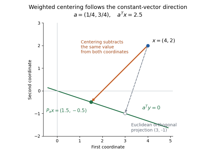
Weighted centering and Euclidean orthogonal projection reach different points on the same zero-weighted-mean line
. Original two-coordinate example with and . The orange arrow subtracts from both components; the dashed arrow is perpendicular to the green line in the Euclidean metric. Details.If every , put . Then , so this same map is orthogonal for the inner product . It is the residual-making map for minimizing over a fitted constant , the intercept-only case of weighted least squares.[ref] Zero weights preserve the algebraic projection but make this proposed inner product degenerate. When all weights equal , the construction reduces to the usual centering matrix.
For a CW complex and coefficient abelian group , the degree- cellular cochain group isChoosing orientations of the -cells identifies it with an arbitrary assignment of one element of to each cell. Since the cellular chain group is a direct sum over cells, the cochain group is a product , which matters when there are infinitely many cells.
The cochain differential is precomposition with the cellular boundary: . The identity gives . In finite cellular bases, its matrix is the transpose of the boundary matrix, interpreted in the coefficient group.
The Casimir energy is the configuration-dependent part of a quantum field's vacuum energy after a specified subtraction or renormalization. Only an energy difference or its derivative is physically meaningful in the idealized calculation; the separate zero-point sums are divergent.
For the electromagnetic field between two infinite perfectly conducting parallel plates at zero temperature and separation , the renormalized energy per area is . Differentiation gives the attractive pressure . Real materials, finite temperature and geometry alter this result. The Casimir effect therefore tests a response to changed boundaries, not a direct weighing of an unregularized infinite energy.
Blank-corrected carbon recovery in polymer tests subtracts measured background carbon from a specimen-containing experiment before comparing recovered carbon with the specimen's initial inventory. It is a carbon-basis closure for polymer degradation calculation with an explicit background model. Uncertainty in that subtraction and differences between blank and specimen conditions both affect the result.
For total measured carbon , mean blank carbon and initial specimen carbon , writeAll terms must use the same carbon-mass or carbon-amount basis. For independent and , ; a shared correction can instead introduce covariance. Uncertainty in also enters the recovery ratio. The GUM's correlated-input rule supplies the general propagation framework.[ref]
An original numerical example measures mg of carbon, with standard uncertainty 0.5 mg. Three independent blank runs give 2, 4 and 6 mg. Their mean is 4 mg, sample standard deviation is 2 mg and estimated standard uncertainty of the mean is mg. Net carbon is therefore 6 mg with standard uncertaintyWith stipulated exact mg, recovery is 25%, with standard uncertainty approximately 5.24 percentage points. A precise total measurement can still leave a relatively uncertain net result after subtraction.
Shared-blank covariance in carbon recovery matters if the same estimated blank corrects several specimens. With independent specimen totals , each corrected quantity is , soFor four specimen totals each having the 0.5 mg standard uncertainty above, averaging the corrected values gives variance . Treating all four corrected values as independent would incorrectly divide the shared blank contribution by four. Taking more specimen readings does not recreate independent blank information.
The OECD 301 B apparatus aerates inoculated medium with carbon-dioxide-free air and measures evolved gas captured in hydroxide traps. Its measured carbon dioxide is corrected for blank inoculum production.[ref] Use matched collection duration, volume and analytical conversion when comparing blanks and specimen vessels; a gas-mass reading must be converted to carbon mass before mixing it with other carbon fractions.
A blank is not guaranteed to reproduce every background process inside the treated vessel. The guideline explicitly notes that endogenous activity in the presence of the test chemical may differ from that in the blank control.[ref] Replication estimates scatter around the blank model; it does not prove additivity. Report the blank design, correction, uncertainty and any evidence for altered background activity alongside the final recovery.
Square-root collapse of capacitive bridging bandwidth near the DC error floor by  Codex 0 2026-11-05
The square-root collapse of capacitive bridging bandwidth near the DC error floor describes how the usable frequency interval disappears when a resistive divider has almost exhausted a complex-error allowance. Use the model and exact formula in capacitive bridging complex-error bandwidth: , , and the DC floor . Write the available extra tolerance as . The exact bandwidth becomesAt fixed positive , the leading numerator is linear in , so is proportional to . Thus demanding four times less extra tolerance approximately halves the bandwidth; it does not reduce it by a factor of four.
For an original example, choose , , and . Then , , and . Taking gives about from the exact formula. Taking gives about . The small deviation from an exact two-to-one ratio comes from the retained quadratic term and denominator.
The qualification fixed positive matters. If the receiving resistance is infinite, andwhich is linear in small . For a small but nonzero floor, the square-root approximation needs small compared with as well as with the remaining distance to unit error. The crossover from square-root to linear capacitive bridging bandwidth scaling prevents using the fixed-floor asymptotic expression uniformly as also tends to zero.
This is a limit of the chosen passive input impedance model, not an empirical limit for every amplifier. The manufacturer's shunt-capacitance model motivates the resistive/capacitive paths; an actual bench comparison must include both amplitude and phase shift and the probe's added capacitance.[ref]
MT-040: Op Amp Input Impedance by Analog Devices. Printed pp. 1–2, Figures 1–2 and Op Amp Input Capacitance
Let be a conformal map that is a bijection between planar domains. Mapping every loop of a Brownian loop soup in by gives a Brownian loop soup of the same intensity in , after changing the clock along each loop. For a Brownian parametrization , the new clock isThe statement concerns unrooted loops: choosing a different starting time on the same loop does not create another object. It follows from conformal invariance of Brownian loop measure and the image property of a Poisson point process.[ref]
For the dilation , spatial lengths multiply by and loop durations by , while the soup intensity parameter stays fixed. Thus the random geometry has no preferred length scale. Keeping the clock change explicit prevents confusing conformal invariance of the loop ensemble with preservation of each loop's original duration.
Bearing thermal stiffness identification uses measured force changes along a specified thermal path, together with independently known expansion behavior, to infer the axial restraint of an assembly. The observed bearing thermal reaction slope is inN/K. Mechanical stiffness is force per displacement, so converting into stiffness requires the free relative-expansion rate in displacement per temperature. In the constant-compliance engaged model,Here and represent the bearing and supporting structure's axial mechanical compliance contributions.
For an original identification example, suppose equilibrated engaged measurements give forces160,320 and480N at temperature increases50,60 and70K. A linear regression gives slope16N/K and, within this model, an extrapolated zero-force engagement increase of40K. If an independent free-expansion measurement gives , the total compliance is and total stiffness is . A16N/K thermal slope is therefore not itself a16N/m spring stiffness.
The measurements have an identifiability limit: the slope determines when is known, rather than determining both contributions separately. A known supporting-structure compliance would imply . Without that extra information, many pairs give the same total. If is also unknown, scaling both and total compliance by the same positive factor leaves the measured slope unchanged.
A bench experiment can measure axial force with a load cell, track shaft and housing temperatures, wait for equilibrated states and fit only measurements from the engaged regime. A separate low-restraint expansion measurement can estimate . Repeating heating and cooling helps test whether friction, changing contact or thermal gradients invalidate the assumed single slope. These are proposed measurement steps, not a claimed manufacturer's experiment. The physical motivation is the need to accommodate relative thermal displacement in a locating/non-locating bearing arrangement.[ref]
Rolling bearings by SKF. Section B.2, printed p.70, thermal expansion and relative axial displacement
For independent and , first-order propagation givesFor with standard uncertainty0.1µm/K and with standard uncertainty0.8N/K, the inferred total compliance has standard uncertainty about0.00884µm/N. Correlated temperature references require the corresponding covariance contribution rather than this independent-input expression.[ref]
Guide to the expression of uncertainty in measurement by JCGM. §5.1.3, sensitivity coefficients; §5.2, correlated inputs
A bearing axial setting tolerance specifies the permitted difference between the realized axial reference position of an assembly and its bearing nominal axial setting. It consumes some of the available bearing axial travel margin. The setting tolerance must therefore be included when deciding whether all required thermal and operating changes remain inside the physical travel limits. The bearing manufacturer's locating/non-locating arrangement discussion explicitly includes relative displacement and accumulated dimensional variation.[ref]
Rolling bearings by SKF. Section B.2, printed p.70, relative axial displacement and tolerance accumulation
Let physical travel be , required displacement changes be , and setting error be . To retain a prescribed margin for every allowed combination, the nominal setting must satisfyThe lower bound follows from the smallest possible realized position ; the upper bound follows from the largest. This is a worst-case guarantee over the stated ranges and needs no assumption that the errors are statistically independent.
For an original example, take , required changes , setting error and required margin0.05mm. The admissible nominal-setting interval is . Choosing gives worst-case operating endpoints and , leaving0.07mm at each end. The asymmetric error range has shifted the balanced nominal setting relative to a symmetric tolerance assumption.
A bearing axial tolerance stack combines the contributing dimensions and their signs before applying this range calculation. Two separate bounded errors of and can add to in the worst case. Taking a square root of summed squares would answer a statistical uncertainty question under additional assumptions; it would not reproduce that deterministic bound. The distinction between a bound and standard uncertainty matters when a guaranteed clearance or reserve is specified.
The resulting interval can be empty. That outcome identifies incompatible travel, operating-change, tolerance and reserve requirements; adjusting the nominal setting alone cannot resolve it. A nonempty interval addresses axial geometry but does not establish acceptable friction, elastic loading or contact conditions after an end stop engages.
Effective beam shear rigidity is the coefficient relating a transverse shear-force resultant to the beam shear angle in a reduced linear beam model:Here is shear modulus, is material area and is a beam shear correction coefficient. The coefficient has units of force, whereas beam flexural rigidity has units . A shear-deformable beam permits section rotation to differ from centreline slope; Bower gives the corresponding force relation and explains the correction coefficient's dependence on section geometry and the approximation used.[ref]
Applied Mechanics of Solids by A. F. Bower. §8.7.2, Summary of beam theory, Timoshenko force relation and shear-coefficient paragraph
An original energy calculation explains one familiar correction. For a homogeneous rectangle of width , thickness and area , adopt the classical parabolic shear-stress approximationIt has resultant . Its shear elastic energy per unit beam length isEquating this to the reduced-model energy gives . Thus follows from this particular energy-matching approximation; it is not a universal material constant or an exact coefficient for every beam theory.
The effect on a three-point bending test can be derived from that reduced energy. For a simply supported beam under central force , the magnitude of shear force is on each half. Hence and its contribution to central displacement is . Combining it with the bending response givesThe shear contribution becomes relatively more important as the span decreases.
For stipulated , , and , the two contributions are and . Shear adds twelve percent of the bending deflection. A span series with a load cell and direct midspan displacement readout can distinguish cubic bending dependence from linear shear dependence, provided contact and fixture contributions are also controlled. Inferring from the response additionally requires the section geometry and correction model.
Gradient accumulation combines gradient contributions from several processed mini-batches before one optimizer update. Parameters stay fixed while those contributions are evaluated. With consistent normalization, an additive per-example loss function can therefore use an effective batch size larger than the group processed at once.[ref]
Automatic Mixed Precision examples in the PyTorch documentation. Gradient accumulation subsection and example loop
For an original example, let per-example scalar gradients be at the same parameter value. Process the first two together and the last separately. Their means are 2 and 8. The combined per-example mean isThe unweighted mean of group means is 5 and gives the smaller group too much weight. One implementation accumulates each group's summed loss divided by the total example count, then performs one update.
Accumulation is also different from consecutive updates. Let , with , starting at and using step size . One accumulated mean-gradient step gives . Updating first on the two-example mean gives ; the last example then has gradient , and a second step gives .
The distinction is where the gradients are evaluated. Agreement with one larger group requires fixed parameters and compatible model state, additive losses and consistent weighting. A method whose calculations depend on the whole group can violate those assumptions. State whether batch size denotes a processed group or the complete set contributing to an update.
An atomic displacement probability level is the fraction of modeled positional probability enclosed by an atomic displacement ellipsoid. It specifies the size of the drawn surface for a given anisotropic atomic displacement parameter; changing the level does not change the fitted displacement matrix.[ref]
Atomic displacement parameter nomenclature (IUCr report). Section2.3.1, constant-probability ellipsoids
For a centered three-dimensional normal distribution with positive-definite Cartesian covariance matrix , defineThe variable has a chi-squared distribution with3 degrees of freedom. To enclose probability , choose satisfying and draw . If are the eigenvalues of , its semiaxis lengths are .
An explicit calculation uses the cumulative distribution functionwhere is the error function. Solving gives ; for , .
For an original comparison, keep . The50% semiaxes are approximately0.154,0.308 and0.461angstroms. The90% semiaxes are approximately0.250,0.500 and0.750angstroms. Every semiaxis grows by the same factor, about1.625, although the underlying directional spread is unchanged.
This also explains why a surface drawn at one root-mean-square displacement in each principal direction, , encloses only about19.9% in three dimensions. The probability inside a three-dimensional ellipsoid differs from the probability inside a one-dimensional standard-deviation interval. Comparisons of displayed atomic sizes therefore need the stated probability levels as well as the displacement parameters.
Exactly-once pin cleanup gives one owner responsibility for ending a particular pinning lifetime, despite several possible completion paths. The resource must remain pinned until its consumers finish, and its cleanup must occur once after that condition is met. This combines the safety requirement of asynchronous pin release with a liveness requirement: a pin left permanently owned by nobody can obstruct later memory compaction.
A useful state machine has states “submission in progress”, “completion pending” and “released”. A submission error that guarantees no future consumer can access the address may take the first state directly to released. A pending result transfers cleanup responsibility to a completion path. Immediate completion must follow the API's stated rule about whether a callback will also arrive; it must not independently trigger two owners to dispose of the same handle. Microsoft's native-call example explicitly handles submission exceptions and funnels immediate or deferred completion into cleanup.[ref]
Memory and Span usage guidelines by Microsoft. Rule10, exception branch, non-pending result branch and completion routine
For an original race example, suppose a completion callback and an error-reporting path can both observe an operation as finished. A plain sequence “test flag; if clear, set flag; release pin” can race: both callers read clear before either writes set, and both release. A synchronized ownership claim, using a mutex or an appropriate compare-and-swap transition, can ensure that only one caller changes pending to released. The losing caller performs no cleanup. This is a schematic ownership protocol, not a claim that every pin API tolerates arbitrary racing callbacks.
For a count of releases on one acquired handle, the at-most-once condition is . The requirement that cleanup eventually occurs after all promised access has ended supplies at final completion, so together they give . A one-time flag alone establishes neither the end of access nor eventual execution of the winning path.
The operation's state must also stay alive while any callback can inspect it. Reference counting can protect that state independently of the pin being released. Marking a handle released does not permit another caller to access freed callback state. Keeping resource ownership, callback-state lifetime and data synchronization separate makes the protocol easier to verify. The primary task-based memory rule similarly requires all consumer access to finish by task termination.[ref]
Memory and Span usage guidelines by Microsoft. Rule4, consumer lifetime through terminal task state
An endpoint certificate for continuous collision clearance uses distances at two sampled configurations and a bound on intervening motion to prove separation for an entire time interval. Its guarantee concerns every intermediate configuration, rather than only the sampled poses.
Let be the set distance between a moving nonempty compact set and fixed nonempty closed set of obstacles, with . Suppose , with , and let the exact endpoint distances be . The two endpoint inequalities implyThis uses a valid clearance Lipschitz continuity constant, such as the rigid-body motion bound derived in angular clearance bound for a rotating body. The continuous-path requirement itself is fundamental to the primary planning model.[ref]
Robotic Systems by Kris Hauser. Chapter 8, Stating the motion planning problem; Chapter 9, rotational configuration-space obstacles
For and consistent endpoint data , the two sloping bounds intersect atTheir maximum is minimized there, giving the sharp general lower boundIt is sharp among nonnegative functions with that Lipschitz continuity bound and those endpoints: the displayed envelope itself satisfies the assumptions. This does not say that the unknown actual trajectory attains the lower bound.
For an original example, take , , and . Since , the simple nearest-endpoint certificate gives . The paired bounds give , with their intersection at . Thus the sharper certificate proves separation greater than a required clearance margin where the simpler one does not.
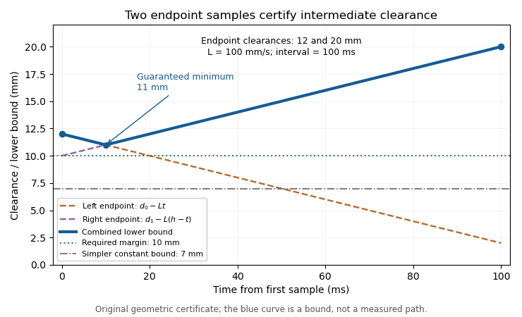
Paired Lipschitz endpoint bounds certify at least 11 mm clearance over 100 ms, while the simpler constant bound gives 7 mm. Original constructed certificate; the blue envelope is not a measured trajectory.
Details. For , consistency requires , and the clearance is constant. An endpoint difference larger than contradicts the exact-data assumptions; the motion bound, query errors or model must be checked. A clearance certificate with bounded distance-query error replaces exact observations with justified lower bounds and must preserve the assumptions used in minimizing their envelope.
Under the strict convention of adaptive clearance sampling, certification requires the guaranteed lower bound to exceed the requested margin. If it does not, unresolved intervals in adaptive collision checking remain undecided until additional queries or other information resolve them. Failure of this sufficient certificate alone does not establish a collision.
Unresolved intervals in adaptive collision checking are trajectory intervals for which the available queries and motion bounds prove neither the requested continuous clearance nor a violation at a known configuration. They are a computational result of incomplete information, rather than evidence that a collision occurred.
In adaptive clearance sampling, suppose endpoint distances and a valid clearance Lipschitz continuity constant are known over an interval of duration . If a lower bound such as does not exceed the required clearance margin, the interval needs further work. Its endpoints can both be clear while its interior remains undecided. The continuous-path requirement motivating this distinction is stated in the primary planning text.[ref]
Robotic Systems by Kris Hauser. Chapter 8, Stating the motion planning problem and Point-to-point path planning
An original indistinguishability example uses , and endpoint clearances . Both of the following functions satisfy the same endpoint data and motion bound:They can be realized by the height of a point moving above a fixed horizontal wall. The first path stays clear; the second reaches the wall. For a requested separation, the initial endpoint certificate is , so the shared endpoint observations cannot distinguish them. A negative lower estimate does not establish a negative physical distance.
Querying the midpoint resolves this constructed example. Model A gives another reading, and each half-interval then has the sufficient bound . Model B gives zero, demonstrating contact. More generally, a strictly positive sampled distance at or below the requested margin establishes a margin violation but not a collision. Exact zero set distance establishes contact or intersection when the modeled body is a nonempty compact set and the obstacles form a nonempty closed set.
If the chosen query, time or subdivision budget expires first, retain the undecided intervals explicitly. Accepting the whole trajectory would discard the unverified portions; labeling every undecided portion a collision would also claim information not obtained.
For exact queries, finite and a true minimum clearance at least with , subdivision eventually yields , making the simple certificate sufficient everywhere. A trajectory merely touching the required threshold has no such surplus. A clearance certificate with bounded distance-query error must also account for how conservative query bounds affect that remaining surplus.
A required clearance margin is the minimum separation requested by a geometric motion specification. In adaptive clearance sampling, it is the threshold that a continuous-interval lower bound must exceed. Positive separation from an obstacle is enough to exclude contact in an exact model, but can still be less than the requested margin.
Let be the modeled nonnegative set distance between a rigid body and fixed obstacles. Using the strict convention of adaptive clearance sampling, an interval is accepted only when its guaranteed lower bound exceeds . A query with violates that requested separation without demonstrating contact. Choosing is part of the specification, not something determined uniquely by the collision detection algorithm.
Geometric uncertainty can be incorporated with explicit bounds. Suppose robot geometry, obstacle geometry and reference-point tracking error can each change the relevant sets by at most in Hausdorff distance. The triangle inequality then givesTo guarantee an actual separation greater than , a sufficient modeled threshold isThese are simultaneous deterministic bounds. No independence assumption is needed to add them conservatively. The configuration-space construction in the primary planning text similarly represents body size by enlarging forbidden regions.[ref]
For an original error budget, require and take geometric bounds of , and respectively. The modeled threshold becomes . Suppose the smaller reported endpoint distance is , the distance-query error is bounded by , the clearance Lipschitz continuity constant is , and the interval duration is . The simple interval certificate givesSubtracting the geometric budget leaves at least actual separation, exceeding the requested by in this model.
The query error was already subtracted from the interval bound and must not be subtracted again as an unrecorded duplicate allowance. Conversely, the motion term addresses unsampled motion; it does not automatically include obstacle-location error. An endpoint certificate for continuous collision clearance should state which effects are included in each quantity, while unresolved intervals in adaptive collision checking retain intervals whose lower bound is insufficient.
Pinned article: Introduction to the OurBigBook Project
Welcome to the OurBigBook Project! Our goal is to create the perfect publishing platform for STEM subjects, and get university-level students to write the best free STEM tutorials ever.
Everyone is welcome to create an account and play with the site: ourbigbook.com/go/register. We belive that students themselves can write amazing tutorials, but teachers are welcome too. You can write about anything you want, it doesn't have to be STEM or even educational. Silly test content is very welcome and you won't be penalized in any way. Just keep it legal!
Intro to OurBigBook
. Source. We have two killer features:
- topics: topics group articles by different users with the same title, e.g. here is the topic for the "Fundamental Theorem of Calculus" ourbigbook.com/go/topic/fundamental-theorem-of-calculusArticles of different users are sorted by upvote within each article page. This feature is a bit like:
- a Wikipedia where each user can have their own version of each article
- a Q&A website like Stack Overflow, where multiple people can give their views on a given topic, and the best ones are sorted by upvote. Except you don't need to wait for someone to ask first, and any topic goes, no matter how narrow or broad
This feature makes it possible for readers to find better explanations of any topic created by other writers. And it allows writers to create an explanation in a place that readers might actually find it.
Figure 1. Screenshot of the "Derivative" topic page. View it live at: ourbigbook.com/go/topic/derivativeVideo 2. OurBigBook Web topics demo. Source. - local editing: you can store all your personal knowledge base content locally in a plaintext markup format that can be edited locally and published either:This way you can be sure that even if OurBigBook.com were to go down one day (which we have no plans to do as it is quite cheap to host!), your content will still be perfectly readable as a static site.
- to OurBigBook.com to get awesome multi-user features like topics and likes
- as HTML files to a static website, which you can host yourself for free on many external providers like GitHub Pages, and remain in full control

Figure 2. You can publish local OurBigBook lightweight markup files to either OurBigBook.com or as a static website.
Figure 3. Visual Studio Code extension installation.
Figure 5. . You can also edit articles on the Web editor without installing anything locally. Video 3. Edit locally and publish demo. Source. This shows editing OurBigBook Markup and publishing it using the Visual Studio Code extension. 
- Infinitely deep tables of contents:




All our software is open source and hosted at: github.com/ourbigbook/ourbigbook
Further documentation can be found at: docs.ourbigbook.com
Feel free to reach our to us for any help or suggestions: docs.ourbigbook.com/#contact