Topics (384k) Articles (398k) Users (410) Discussions (242) Comments (383) Files (13k) New article

A density on a smooth -dimensional manifold transforms under coordinate changes by the absolute value of the Jacobian determinant. If , its local coefficient satisfiesDensities are sections of the corresponding rank-one density bundle. A positive density has positive local coefficient; a general density can have a signed coefficient despite the absolute Jacobian transformation.
A Riemannian metric supplies the positive density . The determinant transformation of the metric matrix gives exactly the required coordinate law. This is the higher-dimensional version of an area density of a surface.
Unlike a top-degree differential form, a density can be integrated without choosing an orientation. A Möbius band therefore has a global positive area density although it has no nowhere-zero global area two-form. The distinction separates integration of unsigned volume from orientation-sensitive integration.
A finite-dimensional quantum dynamical semigroup is Davies irreducible when no proper nonzero subspace can support a state for all future times. Equivalently, if a projection satisfies for every state and every , then or . This is a property of invariant supports, rather than merely uniqueness of a stationary density matrix.
For a two-level system with only spontaneous decay, and zero Quantum Hamiltonian, the ground-state line is invariant. The stationary state is unique but pure, so the dynamics is reducible. Adding a positive excitation rate removes that invariant line; the stationary populations are and and the dynamics is irreducible. In finite dimensions irreducibility ensures a unique faithful stationary state, which has full rank. Related notions of quantum irreducibility must be distinguished.[ref]
Criteria for Davies Irreducibility of Markovian Quantum Dynamics by Yikang Zhang and Thomas Barthel. Sections 3 and 6, invariant supports and two-level examples
For a Lie algebra representation , an invariant vector is a vector annihilated by every represented Lie algebra element:The condition is zero infinitesimal action, not . The invariant vectors form a vector subspace.
For a one-dimensional abelian Lie algebra acting on through , the invariant vectors are exactly the first coordinate line. For the Adjoint representation, invariants are the center of a Lie algebra, because .
If the representation differentiates a representation of a connected Lie group, Lie algebra invariants are also group invariants. Connectedness matters: a disconnected group can act nontrivially even when its Lie algebra acts trivially. The sign action of has zero Lie algebra but no nonzero fixed vector.
A learning rate schedule specifies how the learning rate changes during an iterative learning procedure. Its rule can depend on the update count, a training epoch count or another declared event. The rule and the clock must both be stated: changing a rate every parameter update is different from changing it after a complete pass through the training data.
A simple step-decay example iswhere counts completed schedule advances from zero. The values at are , those at are , and the value at is . The StepLR implementation documents periodic multiplication by a specified factor; its example advances the scheduler after the training and validation operations.[ref]
A different schedule admits an exact convergence calculation. For gradient descent on , take . With no other update terms,Multiplying the successive ratios gives a telescoping product:Starting at gives . This proves convergence for the stated deterministic quadratic, rather than for every objective or noisy learning procedure.
The underlying stochastic gradient descent update also depends on its gradient estimate and any additional terms, not just the scheduled scalar.[ref] Report the initial index, update order and any external changes to the rate. The StepLR documentation explicitly permits other changes alongside its own, so the isolated step formula above assumes that no competing rule intervenes.[ref]
For a random walk with transition matrix , its holding probability at state is , the conditional probability of staying at for the next step. It is the holding probability of a Markov chain specialized to the walk. A lazy random walk can be constructed byIts holding probability is , which equals only if the original walk cannot stay at .
This change preserves every stationary distribution: implies . A positive holding probability permits return in one step, giving period one at that state; for an irreducible Markov chain, this removes periodicity throughout the class. Laziness does not connect previously disconnected classes. For a loop-free walk with , the conventional holding probability is therefore exactly .
The positive constant in layer normalization regularizes division by the coordinate standard deviation. For coordinates, write , and . The normalized core and the full output areHere is the Hadamard product, and are fixed when studying the dependence on . This placement of , the divisor in the coordinate variance, and the elementwise layer-normalization gain and layer-normalization bias define the stabilized convention used here.[ref]
LayerNorm in the PyTorch documentation. Equation; correction=0; Parameters/eps and elementwise_affine
If all coordinates of are equal, then and : positive makes the normalized core well defined and equal to 0, so the full output is .Positive also changes the normalization away from constant inputs. The arithmetic mean of the normalized core is 0, but its normalized coordinate variance in layer normalization isThus it approaches 1 when is large, equals when , and approaches 0 when approaches 0. This formula describes the normalized core; learned, unequal coordinate gains or biases can change the coordinate arithmetic mean and variance of the full output. For , changing from to changes the core from to .
Although layer normalization is invariant under a common input shift, a fixed positive prevents exact positive scaling invariance on a nonconstant input. For ,For and fixed , this equals only when . With , the normalized core is exactly invariant for every wherever . The unstabilized scaling argument in Layer Normalization by Jimmy Lei Ba and others therefore needs this qualification when used for the stabilized formula.[ref]
Layer Normalization by Jimmy Lei Ba and others. §3, equation 3, and §5.1, equations 6–7: normalization statistics and scaling analysis
The same constant controls layer-normalization sensitivity. With the centering matrix , we have , and . Taking a derivative gives the layer-normalization Jacobian:The common-offset vector is an eigenvector with eigenvalue . For , the radial direction has eigenvalue ; a vector orthogonal to both and has eigenvalue . At a constant input, the Jacobian matrix is . These formulas give the operator norm bound for the Euclidean norm. Integrating this derivative along a line segment proves Lipschitz continuity of the normalized core with constant . The bound for the full output is multiplied by , the operator norm of the diagonal matrix of its layer-normalization gain. For , the core bound is attained in centered directions at a constant input: smaller permits larger local amplification near zero coordinate variance.
For the input family , the third coordinate of the normalized core is , with derivative . The dashed lines mark ; the forward response approaches these values for large positive or negative .
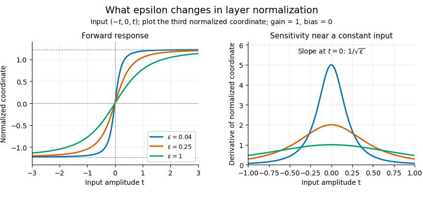
Original layer-normalization response and sensitivity for ; unit gains and zero biases.
Details. Adding the same scalar to every coordinate leaves layer normalization unchanged, provided its layer-normalization gain and layer-normalization bias are held fixed. This is an exact statement even with positive layer-normalization epsilon. Write , let be the coordinate arithmetic mean, and define the coordinate variance . For any scalar , we haveConsequently , so both the numerator and denominator of layer normalization are unchanged. Applying the same coordinatewise layer-normalization gain and layer-normalization bias preserves the equality:The positive layer-normalization epsilon is added to the coordinate variance before taking the square root.[ref]
The centering matrix makes the geometry explicit: and . Thus the common-offset direction lies in the kernel of a linear map represented by . For the normalized core , take and . Its coordinate arithmetic mean is 2 and its coordinate variance is , giving . The vector has exactly the same normalized core. An unequal coordinate shift need not be removed: instead gives .
This identifies a precise redundancy in a neural network. If the vector before layer normalization is an affine map , adding to its bias leaves the normalized result unchanged for every . A shift of the raw input by a vector produces , which need not be a common coordinate shift. The weight re-centering calculation in Layer Normalization by Jimmy Lei Ba and others uses the related transformation : its extra contribution is , which normalization removes separately for each input.[ref]
The layer-normalization Jacobian describes the first-order response of the normalized core to a change in its input. Let be the core defined in layer-normalization epsilon, with . Its Jacobian matrix satisfiesThe closed formula and its derivation are given in layer-normalization epsilon. A matrix entry measures the local effect of changing input coordinate on normalized output coordinate .
An original two-coordinate calculation takes and . Here the centered variance is and the normalized core is . Substitution into the established derivative formula givesConsequentlyThe common-offset direction has no effect; the centered contrast direction changes the output. This is a local linear response, rather than an exact rule for arbitrary finite changes.
For the complete output with fixed layer-normalization gain and layer-normalization bias, the input Jacobian is . In the example, givesThe first output is suppressed, yet the first input still affects the second output. This distinguishes an output gain from removing an input feature. Parameter derivatives with respect to and are separate derivatives. Layer-normalization sensitivity measures the input Jacobian's amplification through an operator norm.
The layer-normalization gain is the learned coordinatewise multiplier applied to the normalized core. With layer-normalization bias , the output is , where is the Hadamard product. The multiplier can differ between coordinates and need not be positive.[ref]
LayerNorm in the PyTorch documentation. 2.15, equation; Variables/weight and Parameters/elementwise_affine
It permits the model to rescale the features after normalization.For an original example, choose and layer-normalization epsilon . The coordinate mean is zero, the coordinate variance is , and the normalized core is . Taking and zero bias givesThe output coordinate arithmetic mean is and its coordinate variance is . Thus the core's centering and variance properties do not automatically survive unequal gains. A negative gain also reverses the sign of its coordinate in this example.
If is the incoming loss gradient, then . For above, the gain gradient is . This concerns a derivative with respect to the learned parameter; the layer-normalization Jacobian instead differentiates with respect to the input with parameters fixed.
Setting one to zero makes that output coordinate equal to its bias, but does not remove input coordinate from the shared normalization statistics. It can still influence other output coordinates through those statistics. The input derivative is obtained by multiplying the core Jacobian on the left by the diagonal matrix of gains. Layer-normalization epsilon contains the general derivative and bound.
The layer-normalization bias is the learned coordinatewise offset applied after the normalized core and layer-normalization gain. Writing the core as ,The offset is a model parameter, rather than an estimate of statistical bias. The PyTorch implementation provides an optional learned additive parameter for each normalized element.[ref]
LayerNorm in the PyTorch documentation. 2.15, equation and Variables/bias; Parameters/bias and elementwise_affine
An original constant-input example isolates its effect. Choose and any positive layer-normalization epsilon. The core is zero, so for the output is exactly , regardless of the fixed gain. Its coordinate arithmetic mean is : the output of the full learned layer need not have zero mean even though its normalized core does.
For a scalar loss with incoming output gradient , the chain rule gives . For the original loss in this example, the bias gradient is therefore . If the same parameter vector is reused at several positions, their gradient contributions add.
An equal shift of every coordinate before normalization is removed, as shown in layer normalization is invariant under a common input shift. The offset here is applied after normalization and persists. When differentiating only with respect to while parameters are fixed, contributes zero to the layer-normalization Jacobian.
The hyperbolic Laplacian is the Laplace-Beltrami operator for the metric of hyperbolic space. In upper-half-space coordinates with ,Using the nonnegative convention givesIndeed, insert and into the coordinate formula . The choice of overall sign must be specified when comparing spectral formulas.[ref]
Analysis on Manifolds via the Laplacian by Yaiza Canzani. section 4.1, Definition 14 and the following local-coordinate formula, printed page 43
In dimension two the first-derivative term disappears. For , direct differentiation gives , and in particular in the hyperbolic plane. This is the eigenvalue expression underlying many Maass form conventions.
Despite its name, this is an elliptic differential operator on : its leading symbol in the chosen sign convention is . The adjective hyperbolic refers to the geometry, not to the classification of a hyperbolic partial differential equation.
Uncertainty in estimated inverse-variance weights arises when the variances used in inverse-variance weighting are themselves estimated. A very small estimated variance can give one observation or group a large random weight. The familiar variance formula for fixed, known weights cannot simply be reused with estimated variances treated as exact. NIST specifically warns that weights estimated from few replicates can substantially and unpredictably affect a weighted least squares analysis.[ref]
Suppose independent groups contain independent normal random variables with common mean and group variance . Let and be the group sample mean and unbiased sample variance, and formFor normal samples, each sample mean is independent of its sample variance. Conditional on the estimated weights, the estimator remains unbiased and hasThus the law of total variance gives unconditional variance equal to the expectation of this expression. The true still appear; replacing them by the same random does not establish the actual conditional variance. Outside the independence assumptions, even conditional unbiasedness can fail.
An original two-group example takes and true , so each group mean has variance . If observed sample variances are and , the estimated normalized weights are and . For group means and , the combined estimate is . The plug-in variance isbut the true conditional variance under the stipulated model isThe corresponding standard deviations are about and . Equal weights would have variance . An accidentally small estimated variance has both overstated precision and moved the combination away from the optimal equal weights in this example.
Reciprocal moments of an estimated variance explain the unstable precision estimate. For a normal sample with , has a chi-squared distribution. Integrating its density givesConsequently for , while the second moment requires . The density and its gamma-distribution parameterization are documented in the primary SciPy implementation notes.[ref] With , the inverse sample variance has a finite mean twice the true precision and an infinite variance; the normalized weights remain bounded, so this does not imply their variance is infinite.
More replication or a justified smooth variance model can stabilize weights. NIST describes direct replicate-based weight estimation and variance-function modeling as distinct approaches.[ref]
Weighted Least Squares by NIST. e-Handbook §4.4.5.2, Direct Estimation of Weights and Estimating Weights with a Variance Function
A proposed validation repeats the complete weight-estimation and combination procedure on simulated or replicated groups, checking actual interval coverage as well as point estimates. A bootstrap must reproduce the weight-estimation stage; holding the fitted weights fixed tests a different procedure.A reset error budget with a persistent pedestal assigns separate tolerance to a decaying pre-reset residual and an offset created when the reset switch opens. Increasing the preceding discharge time can reduce the former without reducing the latter. The integrator reset settling time article derives the basic worst-case bound and its logarithmic reset-duration requirement.
A focused extension includes leakage during a fixed post-opening readout delay . Let the pre-reset residual magnitude be at most , its decay time constant be , the opening reset charge-injection pedestal magnitude be at most , and subsequent electric current magnitude be at most on fixed capacitance . The triangle inequality givesThis separates a duration-controlled term from an error floor . For and a required guarantee , finite reset time is possible from this bound only when , and
For an original chosen circuit, take , , , , and . Leakage consumes . A total tolerance leaves for the old residual, requiring about of reset. A tolerance requires changing the stipulated pedestal or readout conditions; reset duration alone cannot guarantee it.
These are worst-case bounds, not root-sum-square standard uncertainties. Test the discharge by varying , the opening step with zero-input records, and the subsequent drift by varying . Real charge transfer depends on switching sequence, and prior overload can require separate recovery.[ref]
ACF2101 Low Noise, Dual Switched Integrator datasheet. p11, Charge Transfer and Droop; p10, Output Overload
Accidental cancellation of signed errors is not a reproducible worst-case margin.Phase calibration error in an admittance-based capacitance estimate can rotate a large in-phase conductance into a small capacitive quadrature. In the parallel port model with , , and the convention, a relative wave phase error gives . The exact estimate in input capacitance inferred from measured admittance therefore has relative errorThe ratio , not the DC resistance alone, determines sensitivity to a small wave phase rotation. The manufacturer's separate differential/common-mode port models motivate specifying the terminals and operating point before fitting an input capacitance.[ref]
MT-040: Op Amp Input Impedance by Analog Devices. Printed pp. 1–2, Figure 1 and Op Amp Input Capacitance
If , the worst absolute relative error is bounded byThe negative endpoint attains this bound. For target relative error , a sufficient frequency condition isThis condition assumes the same model and the same phase-error bound remain valid over that frequency range.
For an original planning example, take , and . The bound is about at and at . A one-percent target requires approximately in this model. Increasing frequency suppresses the conductance-mixing term, but leaves the term and can expose other unmodelled parasitic effects.
A measurement uses the same voltage/current wave phase reference for the ratio , checks that reference with a known port, and retains fixture admittance in the model or subtracts a validated value. Amplitude measurement calibration alone cannot establish this wave phase bound. The numbers above are chosen calculations, not device specifications or a claim that a high-frequency measurement is automatically more accurate.
Overhung idler loading occurs when an idler gear's mesh resultant acts outside the axial span of its shaft supports. The overhang creates a lever arm, so the nearer mechanical bearing can carry a larger transverse load than the mesh resultant and the farther support can have the opposite reaction direction. This geometry is separate from whether the idler's two transmitted torques cancel.[ref]
Place ideal radial supports A and B at and . An upward mesh resultant at , with overhang , gives static equilibriumHenceFor , and , A acts upward with60N while B acts downward with260N. Their signed sum balances the applied200N. The larger reaction at B is a lever effect, not an additional external mesh force.
The overhung shaft bending moment immediately next to the near support has magnitude in this ideal model. That bending moment can exist while the net shaft-axis torque on the steady idler is zero. Doubling overhang at fixed load doubles the near-support bending moment and changes the reaction magnitudes to120 and320N.
Idler bearing load sharing must therefore include the gear's axial position, not just its pitch radius and speed ratio. Loads in independent transverse directions can be balanced separately and then combined as vectors. A support model with more constraints requires compatible deformations as well as force balance. Shaft bending and support flexibility can also alter the gear face load distribution, linking the overhang geometry to tooth loading.
The holding rate at state of a continuous-time Markov chain with generator matrix isFor a conservative chain with finite , its holding time has exponential distribution: and . Conditional on a jump, the next state is with probability . Thus the rate determines when departure occurs, while normalized outgoing rates determine where it goes.
If the outgoing rates are and for two distinct other states, the total rate is five, the mean holding time is , and departure chooses them with probabilities and . A zero rate gives an absorbing state with infinite holding time. Statewise finite rates alone do not rule out explosion of a continuous-time Markov chain.
A Hamiltonian diffeomorphism is the time-one map of a Hamiltonian isotopy beginning at the identity on a symplectic manifold. The isotopy is generated by a smooth time-dependent Hamiltonian function . Its flow must exist for the whole interval; on an open manifold a common group convention requires compact support throughout that interval.
In the convention , the infinitesimal preservation law isThus every Hamiltonian diffeomorphism is a symplectomorphism. The conclusion follows from closedness of the symplectic form, not from a special choice of coordinates.
The identity is generated by the zero Hamiltonian. Inverses and compositions are again Hamiltonian endpoints, forming the group of Hamiltonian diffeomorphisms. A generating function path and its endpoint are different data: different isotopies can have the same time-one map. The Hamiltonian condition imposes more structure than only preserving the symplectic form.
The argmax of a function is the set of inputs where its largest value is attained:It records global maximizers, whereas records the value. For , the argmax on is and the maximum value is zero. If is constant, every input belongs to the argmax.
The argmax can be empty: on has supremum one but never attains it. A continuous function on a nonempty compact set does attain its maximum by the extreme value theorem. Writing a single input as an argmax therefore implicitly assumes uniqueness or specifies a rule for choosing between ties. This distinction matters when an optimization problem is used to define an estimator.
Pinned article: Introduction to the OurBigBook Project
Welcome to the OurBigBook Project! Our goal is to create the perfect publishing platform for STEM subjects, and get university-level students to write the best free STEM tutorials ever.
Everyone is welcome to create an account and play with the site: ourbigbook.com/go/register. We belive that students themselves can write amazing tutorials, but teachers are welcome too. You can write about anything you want, it doesn't have to be STEM or even educational. Silly test content is very welcome and you won't be penalized in any way. Just keep it legal!
Intro to OurBigBook
. Source. We have two killer features:
- topics: topics group articles by different users with the same title, e.g. here is the topic for the "Fundamental Theorem of Calculus" ourbigbook.com/go/topic/fundamental-theorem-of-calculusArticles of different users are sorted by upvote within each article page. This feature is a bit like:
- a Wikipedia where each user can have their own version of each article
- a Q&A website like Stack Overflow, where multiple people can give their views on a given topic, and the best ones are sorted by upvote. Except you don't need to wait for someone to ask first, and any topic goes, no matter how narrow or broad
This feature makes it possible for readers to find better explanations of any topic created by other writers. And it allows writers to create an explanation in a place that readers might actually find it.
Figure 1. Screenshot of the "Derivative" topic page. View it live at: ourbigbook.com/go/topic/derivativeVideo 2. OurBigBook Web topics demo. Source. - local editing: you can store all your personal knowledge base content locally in a plaintext markup format that can be edited locally and published either:This way you can be sure that even if OurBigBook.com were to go down one day (which we have no plans to do as it is quite cheap to host!), your content will still be perfectly readable as a static site.
- to OurBigBook.com to get awesome multi-user features like topics and likes
- as HTML files to a static website, which you can host yourself for free on many external providers like GitHub Pages, and remain in full control

Figure 2. You can publish local OurBigBook lightweight markup files to either OurBigBook.com or as a static website.
Figure 3. Visual Studio Code extension installation.
Figure 5. . You can also edit articles on the Web editor without installing anything locally. Video 3. Edit locally and publish demo. Source. This shows editing OurBigBook Markup and publishing it using the Visual Studio Code extension. 
- Infinitely deep tables of contents:



All our software is open source and hosted at: github.com/ourbigbook/ourbigbook
Further documentation can be found at: docs.ourbigbook.com
Feel free to reach our to us for any help or suggestions: docs.ourbigbook.com/#contact