The knife clearance angle is the angle between the blade face facing the newly cut specimen surface and that surface, measured in the cutting cross-section. It describes how the knife is oriented. The knife wedge angle instead describes the angle between the two blade faces at the edge. Tilting the holder changes clearance without changing the blade's intrinsic wedge geometry.^[ref]

Positive clearance lets the trailing blade face move clear of the cut surface. With insufficient clearance, that face can press or rub against the specimen instead of clearing it. Excessive tilt changes the cutting geometry too; simply maximizing clearance is not a general route to an undistorted section.^[ref]

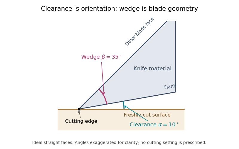
For the ideal straight faces in the diagram, let $\alpha$ be clearance and $\beta$ the wedge angle. Their upper-face orientation relative to the cut surface is $\alpha +\beta$. With the chosen $\alpha =10^{\circ }$ and $\beta =35^{\circ }$, it is $45^{\circ }$. Tilting the whole blade by $3^{\circ }$ gives clearance $13^{\circ }$ and upper-face orientation $48^{\circ }$, while $\beta$ stays $35^{\circ }$.

There is also a simple gap calculation. A point a projected distance $x$ behind the cutting edge lies $h=x\tan \alpha$ above the ideal cut plane. At $x=1\mu \mathrm{m}$ and $\alpha =10^{\circ }$, $h\approx 0.176\mu \mathrm{m}$. Real bevels and specimen deflection complicate this geometry, and the holder's indicated angle must be interpreted using its manufacturer's convention. Comparing section compression and surface defects at otherwise matched conditions can test the consequences of an angle change; the angle scale alone is not a measurement of section quality.

For a continuous map $f:X\to Y$ and a sheaf $\mathcal{F}$ of abelian groups, the higher direct image sheaf $R^q{f}_{\ast }\mathcal{F}$ is the $q$th right derived functor of the direct image sheaf construction. An injective resolution $\mathcal{F}\to I^{\bullet }$ givesEquivalently, it is the sheafification of the presheaf $V\mapsto H^q(f^{-1}(V),\mathcal{F})$ on open subsets of $Y$. Sheafification matters: those higher cohomology groups need not already satisfy the sheaf gluing axiom as a presheaf.

At $q=0$ this is the ordinary direct image $f_{\ast }\mathcal{F}$. If $Y$ is a point, higher direct images are the ordinary sheaf cohomology groups of $X$, regarded as sheaves on that point. For the identity map, every higher direct image with $q>0$ vanishes because the identity direct-image functor is exact.

For a family of schemes, these sheaves organize cohomological information over the base. Their comparison with cohomology on individual fibers is the subject of cohomology and base change, whose hypotheses control when that comparison is valid.

A current-sign certificate for an averaged sensor sample bounds the difference between a filtered current reading and the actual electric current throughout a future switching interval. An average is a weighted history, so it cannot automatically be treated as an instantaneous reading at the end of its acquisition window. This matters for current-polarity dead-time compensation, whose current-path model can fail if the actual current crosses zero during the interval. The physical recirculation paths are documented in the manufacturer’s bridge-switching diagrams.^[ref]

Let an averaging window end at $t_b$ and have age coordinate $a\in [0,T_a]$. Suppose the reported reading isAssume $|di/dt|\le L_i$ over the acquisition history and target interval ending at $t_e\ge t_b$. If $k\ge 0$, then for every future $t\le t_e$,where $\bar{a}={\int }_0^{T_a}ak(a)da$ is the mean sample age. The triangle inequality and the derivative bound prove this result; nonnegative normalized weights make it a convex average. A positive sign is certified by $i_m>b$, and a negative sign by $i_m<-b$, with $b$ the boxed quantity.

Uniform averaging gives $\bar{a}=T_a/2$. A triangular weighting favoring recent values, $k(a)=2(1-a/T_a)/T_a$, instead gives $\bar{a}=T_a/3$. For an original comparison, take $T_a=6\mu \mathrm{s}$, $t_e-t_b=2.5\mu \mathrm{s}$, $L_i=5000A/s$ and ${ϵ}_i=0.020\mathrm{A}$. The uniform bound is $0.0475\mathrm{A}$; the triangular bound is $0.0425\mathrm{A}$. A $0.0450\mathrm{A}$ reading certifies positivity only under the triangular model, leaving a $0.0025\mathrm{A}$ lower margin. This comparison holds the error bound fixed; changing a real filter can also change noise and calibration errors.

Timestamp uncertainty enlarges the age budget. If the actual window could end another $\delta t$ earlier than reported, use $t_e-t_b+\delta t$ in the bound. Any uncertain output scheduling or gate delay likewise belongs in the latest possible target end time. These are bounds on the complete timing relation, not just the controller’s nominal sampling period.

A signed-filter current-sign certificate needs a different expression when a reconstruction filter has negative coefficients. The safe bound isNormalization alone does not justify replacing this by a mean age. For the two-tap estimate $i_m=2i(t_b)-i(t_b-T_a)$, the weighted timestamp lies in the future, but the estimate is not a future measurement. At $t=t_b$, the general bound is $L_i{T}_a$ before sensor error, and a current ramp can attain it. A naive negative-age bound would give a false certificate.

A proposed validation applies known ramps and switching waveforms while recording the acquisition weighting, timestamps and independent current trace. Test the claimed derivative and sensor-error bounds over the whole contributing history. Infinite-memory filters require a bounded contribution from the unobserved tail or a justified history assumption. A successful certificate excludes a zero under its assumptions; a failed one leaves the interval undecided rather than proving a sign reversal.

The CSS initial scroll position is the alignment of a CSS scroll container's scrollable overflow rectangle within its CSS scrollport before scrolling operations take effect. It depends on the applicable layout rules. It usually coincides with the CSS scroll origin alignment, but the two are distinct concepts.^[ref]

Take a $600$-pixel-wide content strip viewed through a $200$-pixel-wide scrollport. Use physical coordinates increasing from the content's left edge, no transforms and ordinary horizontal flow. If the initial alignment is the default origin alignment with inline-start on the left, the view covers $[0,200]$. If inline-start is on the right and origin alignment applies, it covers $[400,600]$. Both can be initial origin-aligned views under the respective stated directions; physical left-edge coordinates do not identify a universal API offset.

A CSS writing mode supplies part of the directional context. Other layout and scrolling features can adjust the initial alignment. The pinned overflow draft explicitly gives CSS scroll snapping as an example that can make the initial position differ from origin alignment. Inferring the initial position solely from a physical corner would miss that qualification.^[ref]

A later scrolling operation is a different event. In the first numerical example, moving to offset $200$ exposes $[200,400]$ under the stated coordinates, while the content dimensions stay fixed. The visible position has changed; this does not redefine the earlier initial alignment. A script that scrolls before a user interacts can likewise change what the user first sees, so the first observed frame alone need not reveal the specification's pre-operation position.

For programmatic inspection, use the coordinate rules of the relevant scrolling interface. CSSOM View Module by World Wide Web Consortium defines element members such as scrollLeft and their relation to the scrolling area's alignment. Distinguish that numerical convention from the layout's geometric CSS initial scroll position before interpreting an observed value.^[ref]

A weighted coverage function assigns nonnegative weights $w_u$ to members of a finite universe $U$, lets each choice $i$ cover a subset $A_i\subseteq U$, and values a selection $S$ byAn item covered twice is counted only once. If $A_1=\{a,b\}$, $A_2=\{b,c\}$ and the weights are $2,3,5$, then $f(\{1\})=5$, $f(\{2\})=8$ and $f(\{1,2\})=10$.

Its marginal gain of a set function is the total weight of newly covered items. As the selected set grows, fewer uncovered items remain, so the marginal gain of a set function can only decrease. This proves that a weighted coverage function is a monotone submodular set function. Nonnegative weights are essential to this argument. The construction models selecting sensors or experiments whose observations overlap.^[ref]

For real random vectors $\mathbf{a}\in {\mathbb{R}}^p$ and $\mathbf{b}\in {\mathbb{R}}^q$ with finite second moments, their cross-covariance matrix collects the covariances between the two sets of coordinates:It has size $p\times q$, and exchanging the two vectors transposes it: $C_{ba}=C_{ab}^T$. Unlike a covariance matrix of a vector with itself, a cross-covariance matrix need not be square or symmetric.

For an original construction, let centered independent random variables $X,Z$ have variances1and4, and putLinearity of covariance givesThe second entry contains a negative contribution from $Z$, although the total is positive. Also $\mathrm{Var}(b)=13$ andThis joint covariance matrix is positive semidefinite. That restriction couples its diagonal and off-diagonal blocks; an arbitrary rectangular matrix cannot be combined with arbitrary within-vector covariances to produce a valid joint model.

For fixed real matrices $A,B$ and constant vectors $c,d$, direct substitution into the definition givesThis identity propagates shared input fluctuations through two different linear readouts, for example when assessing shared calibration error.

From $n$ independent identically distributed paired observations, the usual unbiased estimate isThe pairing must be preserved: independently shuffling the second set changes the estimated association. NIST's multivariate tutorial gives the coordinate sample-covariance formula and its assembly into a covariance matrix; the rectangular formula above is the block joining the two chosen coordinate groups.^[ref]

Every real symmetric matrix $\Sigma$ satisfying $a^T\Sigma a\ge 0$ for every real vector $a$ is the covariance matrix of a random vector taking only finitely many values. The stated inequality means that $\Sigma$ is a positive semidefinite matrix. One does not need a multivariate normal distribution to realize a specified second-moment geometry. Conversely, a proposed covariance matrix must be positive semidefinite, since $a^T\Sigma a$ is the variance of the projection onto any real vector $a$.

Here is an explicit construction. If $r$ is the matrix rank of $\Sigma$, orthogonal diagonalization gives a real $d\times r$ matrix $L$ withLet $S_1,\dots ,S_r$ be independent Rademacher random variables, each equal to $-1$ or $1$ with probability $1/2$, and put $S=(S_1,\dots ,S_r{)}^T$. Then $\mathbb{E}S=0$ and $\mathbb{E}[S{S}^T]=I_r$, soThe random vector $E$ has at most $2^r$ possible values. Adding any constant vector $\mu$ prescribes its mean without changing its covariance matrix. If $r=0$, the constant vector alone suffices.

For an original two-dimensional example chooseThe four equally likely values of $E$ areTheir coordinate means vanish. Their squared first coordinates average to $4$, their squared second coordinates to $(9+1+1+9)/4=5$, and their coordinate products to $(6-2-2+6)/4=2$. The displayed covariance matrix is therefore realized exactly, without sampling error or an asymptotic argument.

These four values are a complete probability model with masses $1/4$, not automatically an independent random sample whose population is unknown. Applying the usual divisor-three sample covariance matrix to the same four rows would give $4\Sigma /3$. NIST explicitly distinguishes that unbiased sample formula with divisor $n-1$; probability-weighted population moments use the assigned masses instead.^[ref]

The sign construction need not minimize the number of points. If a distribution has $m$ positive-mass support points, the centered points obey one nontrivial weighted relation, so their span has dimension at most $m-1$. Its covariance matrix consequently has matrix rank at most $m-1$, requiring $m\ge r+1$ when $r>0$. Matching a covariance matrix also does not match the full probability distribution: this finite model and a continuous Gaussian model can have identical means and covariances while assigning very different probabilities to nonlinear events.

Inception is a family of convolutional neural network architectures built around modules with parallel processing branches. An early module combines several convolution sizes and a pooling layer, then joins their outputs along the channel dimension. Pointwise convolution can reduce channel counts before more expensive spatial operations.^[ref]

For a stipulated shape example, let every branch produce a $28\times 28$ grid, with output channel counts $64$, $128$, $32$ and $32$. Joining channels gives a $28\times 28\times 256$ output becauseThe equal spatial grid sizes are an assumption ensured by the branch design. Channel joining does not add corresponding values into one channel; it retains the distinct branch outputs as separate channels of the combined neural network feature map.

A cost example explains the reduction branch. Ignoring biases, a dense three-by-three convolutional layer from $192$ input channels to $128$ output channels hasweights. Reducing first from $192$ to $32$ channels with a one-by-one pointwise convolution, then applying the three-by-three layer, usesweights. This own example isolates channel dimensions; it is not a reported layer configuration or a claim that the two computations represent identical functions.

The original paper presents this design in the GoogLeNet network and evaluates image classification and detection. Later Rethinking the Inception Architecture for Computer Vision by Christian Szegedy and others develops additional factorization and training choices. The family name therefore does not identify one immutable list of layers or one universal performance result.^[ref][ref]

A convolutional layer applies shared local filters across an input grid to produce output neural network channels. Each filter combines the input channels and nearby positions, with the same learned weights reused at different output positions. This weight sharing distinguishes it from assigning unrelated weights to every grid location.^[ref]

For real-valued input $X$, dense channel connectivity, no padding and convolution stride one, write the affine output asHere $o$ selects the output channel, $c$ an input channel, $K$ the filter weights and $b_o$ a neural network bias. The spatial indices stay in range. This unflipped-filter formula is the cross-correlation convention used by the Conv2d implementation, despite its convolution name. Mathematical discrete convolution reverses the kernel's displacement indices; state the convention when comparing formulas.^[ref]

For one input channel, takeThe first patch gives $1+2(5)-15=-4$. Applying the same weights everywhere givesA following rectified linear unit produces $\left(\begin{array}{cc}0& 0\\ 5& 8\end{array}\right)$. The affine filter operation and the subsequent activation function are separate steps, although an architectural description sometimes groups them together.

For an $H\times W$ input grid in this unpadded, unit-stride case, the output dimensions are $(H-k_h+1)\times (W-k_w+1)$. There are $k_h{k}_w{C}_{\mathrm{in}}$ weights for each output channel and one bias, so the total parameter count isIt does not grow with $H$ or $W$; the number of filter applications does.^[ref]

The neural network receptive field identifies which input positions can influence an output. Local filters restrict that dependency, while successive layers can combine information from a larger region. Convolution stride and zero padding alter the spatial sampling and boundary behavior; the explicit formulas above assume neither subsampling nor padding.

A neural network feature map records a network's responses across positions in its input or an intermediate grid. In a convolutional neural network, one common convention calls each output neural network channel a feature map; several such maps are stacked to form the layer's output. State whether the phrase denotes one channel or the collection, since both usages occur.^[ref][ref]

For an own example, use the single-channel gridApply a two-by-two local averaging filter without padding and with convolution stride one. Its output map isA second filter subtracting each patch's left column from its right column givesFor example, its upper-left response is $(2+5)-(1+4)=2$. The two maps describe different local properties of the same input.

Stacking $A$ and $D$ gives an output with two neural network channels, each on a two-by-two grid: $2\times 2\times 2$ values in channel-height-width order. The channel index identifies which response rule was used; it is distinct from either spatial index. An activation function can then transform those values before another convolutional layer processes them.

The hand-chosen filters make the example interpretable, but learned maps need not correspond to a human-named object or property. Their entries are numerical responses determined jointly by the input, weights and preceding computation. A neural network feature map also need not have the same spatial dimensions as its input: patch size, convolution stride and padding affect the grid. Keeping the channel and spatial axes separate helps interpret both the computation and its dimensions.

A neural network receptive field describes which input positions can influence a specified output unit through the network's computational connections. A local convolutional layer uses only a small input region for each output, but successive layers can combine information from a larger region. This dependence is relative to a chosen input layer; an immediate previous-layer neighborhood and the corresponding original-input region have different sizes.^[ref]

For an own one-dimensional example, use two kernel-size-three convolutional layers, with convolution stride one, no padding and no convolution dilation. Intermediate units $0$, $1$ and $2$ depend on input sets $\{0,1,2\}$, $\{1,2,3\}$ and $\{2,3,4\}$ respectively. The first output of the second layer combines these three units, so its possible original-input dependency isTwo size-three filters therefore give a size-five receptive region, not size nine.

A recurrence tracks the geometry of an undilated serial network. Let $r_{\ell }$ be the span of the receptive region in original-input positions and $j_{\ell }$ the original-input index separation between adjacent layer-$\ell$ outputs. With kernel size $k_{\ell }$, stride $s_{\ell }$ and initial values $r_0=j_0=1$,The last contributing previous-layer unit lies $(k_{\ell }-1)j_{\ell -1}$ input positions beyond the first, which proves the span increment. This derivation assumes the stated local serial connectivity, no padding and no dilation.

If the first size-three layer instead has stride two, then $r_1=3$ and $j_1=2$. A second size-three, stride-one layer has $r_2=7$: its three input supports are $\{0,1,2\}$, $\{2,3,4\}$ and $\{4,5,6\}$. Their union reaches from zero through six. For other sampling choices, a span can include gaps, so span and number of contributing positions need not agree.

This is a structural dependency calculation. Zero weights or the current behavior of an activation function can suppress an influence that the architecture permits; the calculation does not measure how strongly each position affects a particular output. A unit-stride pointwise convolution mixes neural network channels at the same location and does not enlarge this spatial region. The distinction helps explain why many channels alone do not guarantee access to distant input context.

The tail assumptions needed for conservative Wald coverage concern the distribution of the standardized estimation error and the realized scale of its interval. An expected-value bound on a conservative variance estimator does not establish either property. The discrete and rare-large-variance counterexamples in conservative variance estimation does not guarantee Wald interval coverage isolate those failures. NIST similarly makes a normal-model qualification before interpreting an expanded uncertainty as approximately 95 percent coverage.^[ref]

A precise sufficient asymptotic argument is the following. Let $V_n={\mathrm{Var}}_{\theta }({\hat{\theta }}_n)>0$, take ${\hat{V}}_n\ge 0$, and supposeThe first condition includes centring at the true parameter; asymptotically material bias would change it. The second condition is convergence in probability of a variance ratio, substantially more than an expectation inequality. By Slutsky's theorem, the Wald confidence interval with normal critical value $z={\Phi }^{-1}(1-\alpha /2)$ then has limiting coverage probabilityThe limiting normal distribution has no mass on the interval boundary, which justifies passing to that probability. This is asymptotic conservative Wald coverage under variance-ratio convergence, not a finite-sample guarantee.

For an original exactly normal comparison, let a sample mean have true variance $V_n$ and use the deterministic scale ${\hat{V}}_n=1.44V_n$. A nominal 95 percent Wald confidence interval uses a radius $1.2$ times the usual one and has exact coverage probability $2\Phi (1.2\times 1.959964)-1\approx 0.9813$. The calculation uses an actual normal sampling law and a fixed ratio; it cannot be inferred from $E{\hat{V}}_n\ge V_n$ alone. The normal cdf and inverse-cdf implementations provide the numerical evaluation.^[ref]

A samplewise variance upper bound supplies a separate finite-sample route when the centre is exactly normal, because each reported interval contains the known-variance normal interval. Without that shape assumption, use a justified tail inequality as in confidence bounds from a samplewise variance bound.

The conductance profile records bottlenecks at different stationary sizes in a finite irreducible Markov chain with at least two states. With stationary distribution $\pi$ and stationary flow $Q(x,y)=\pi (x)P(x,y)$, one convention isThis domain ensures that the minimizing family is nonempty. Other normalizations use the smaller side of a cut, so a convention must accompany a quoted profile.

For a lazy nearest-neighbor walk on an $n$-cycle, holding with probability $1/2$, a consecutive block of $k\le n/2$ vertices has boundary flow $1/(2n)$ and stationary mass $k/n$, hence conductance $1/(2k)$. A profile therefore reveals how bottlenecks change with set size rather than retaining only one global minimum.^[ref]

Self-complementary RNA duplex melting dissociates a duplex formed by two copies of the same RNA strand into separate strands. Self-complementarity means that the strand's reverse complement can match its own nucleotide sequence. The reaction has molecularity two in the association direction, unlike intramolecular RNA hairpin melting.

Use the ideal association model $2S\rightleftharpoons D$. Let total strand molar concentration be $c_T=[S]+2[D]$ and paired-strand fraction be $f=2[D]/c_T$. With reference molar concentration $c^{\circ }$, the dimensionless equilibrium constant isSubstituting $[S]=c_T(1-f)$ and $[D]=f{c}_T/2$ givesThe final expression is the physical solution for a self-complementary RNA duplex population; the algebraically equivalent subtractive form loses numerical precision at small $\alpha$.

At $\alpha =1$, half the strands are paired. For an original $c_T=10\mu \mathrm{M}$ example, this means $[D]=2.5\mu \mathrm{M}$ and $[S]=5\mu \mathrm{M}$. Duplexes are only one-third of the independently diffusing molecular objects, $[D]/([D]+[S])=1/3$. Half the strands is not half the objects. At fixed temperature and $K_a$, increasing $c_T$ tenfold makes $\alpha =10$ and $f=0.8$.

Heating changes $K_a$ and thus the population. At the strand-based midpoint, $K_a(T_m)=c^{\circ }/c_T$, which explains the concentration dependence of RNA melting. A fit should state whether its constant describes association or dissociation and whether concentration counts strands or duplexes.

Real sequences can also form competing hairpins. A primary tetraloop study explicitly compared predicted hairpin and duplex equilibria when designing its optical-melting sequences.^[ref] The equations above assume only separated strands and duplexes; they do not automatically cover competing folds or RNA melting hysteresis.

Pleural-pressure calibration and compensating component errors arise when an internal-pressure estimate partitions total respiratory stiffness into lung and chest-wall contributions. A gain or offset error can shift those inferred components in opposite directions while their sum still agrees perfectly with the measured total.

An original local model treats the volume increment $\Delta V$ as known. Let true pleural-pressure change be $\Delta P_{\mathrm{pl}}$ and the measured surrogate beHere $k$ is gain and $d$ is an offset change between the two volume states. With wall elastance $E_W=\Delta P_{\mathrm{pl}}/\Delta V$ and known total elastance $E_T$, inference givesThus the component errors are equal and opposite. A constant absolute pressure offset cancels when taking increments, but a changing offset or gain error remains.

For stipulated $\Delta V=0.5$ L, total pressure increment 5 cm water and true pleural increment 2 cm water, the true component elastances are $E_W=4$ and $E_L=6\mathrm{cm}{\mathrm{H}}_2\mathrm{O}{\mathrm{L}}^{-1}$. A surrogate gain $k=1.5$ with $d=0$ instead gives 6 and 4. Checking only their sum cannot identify the measurement calibration error. The GUM requires uncertainty and correlations from shared measurement calibration inputs to remain in the measurement model.^[ref]

The esophageal balloon occlusion test supplies an experimental constraint. In the 1982 primary study, Ahmet Baydur and colleagues measured changes in esophageal and mouth pressure during inspiratory efforts against an occluded airway in ten subjects and several postures. Pressure-change ratios were near unity in sitting and lateral positions; some supine discrepancies could be reduced by repositioning the balloon.^[ref]

The underlying mechanical argument is that an ideal occlusion effort with negligible volume change produces negligible change in elastic transpulmonary pressure. Mouth and pleural pressure changes should then track each other. Comparing the recorded changes tests pressure transmission under those conditions. It does not by itself identify an absolute pressure zero or establish that one position represents every regional pleural pressure during all breathing states. The measurement, its validation maneuver and the inferred elastic partition therefore remain distinct pieces of evidence.

Reactive power is the imaginary part of complex electrical power in sinusoidal steady operation. With RMS phasors, the passive sign convention and $e^{j\omega t}$ time convention,where $\phi$ is potential-difference phase minus current phase. Inductive current lag gives positive $Q$, while capacitive current lead gives negative $Q$. Its conventional unit is the reactive volt-ampere, written var. These definitions retain the specified phasor and sign conventions.^[ref]

The physical role is periodic energy exchange rather than an additional dissipated-energy average. For an ideal inductor, $v=Ldi/dt$ and stored energy is $w=L{i}^2/2$, so $p=dw/dt$. Its energy returns to its initial value after a steady cycle and mean absorbed power is zero. Nevertheless,For an ideal capacitor, $Q_C=-\omega C{V}_{\mathrm{rms}}^2$, with the negative sign representing the opposite exchange phase. Primary circuit derivations explicitly separate these exchanges from resistor dissipation.^[ref]

For an original example, $L=20\mathrm{mH}$, $I_{\mathrm{rms}}=5\mathrm{A}$ and $f=50\mathrm{Hz}$ give $Q_L\approx 157.08\mathrm{var}$. Peak stored energy is0.50J and mean stored energy0.25J, consistent with $2\omega ⟨w⟩$. Zero ideal average dissipation therefore does not mean zero current or zero energy storage.

For a separate ideal single-frequency compensation example, a100V load with $S=400+j300\mathrm{VA}$ can have its source reactive component canceled by a parallel capacitor satisfyingThe capacitor contributes $-j300\mathrm{VA}$, leaving400W of source active power and4A RMS source current. This illustrates power factor correction under the stated ideal assumptions, rather than selecting a real component or proving its ratings.

Reactive exchange can increase the current carried through resistive wiring and thereby affect real losses. For distorted waveforms, definitions of non-active power need additional care; the one-frequency imaginary-part definition should not silently be extended to every waveform.

Apparent power is the product of RMS terminal electric potential difference and electric current, conventionally expressed in volt-amperes:For sinusoidal signals at one frequency, it equals the magnitude $|S|$ of complex electrical power and satisfies $S_{\mathrm{app}}^2=P^2+Q^2$. It is not generally the average rate of net energy absorption, which is active power.^[ref]

For an original example, a100V terminal pair carrying5A RMS has500VA of apparent power. If active power is400W, the power factor is0.8. In the sinusoidal case the magnitude of reactive power is $\sqrt{500^2-400^2}=300$ reactive volt-amperes; the magnitude calculation alone does not determine whether the current leads or lags.

Magnitudes do not add like complex quantities. Consider two parallel sinusoidal loads at the same supply, with complex powers $300+j400$ and $300-j400$ in volt-amperes. Each has500VA of apparent power, but the combined terminal complex power is600VA with zero imaginary part. The source therefore sees600VA rather than the1000VA sum of individual magnitudes. Their internal branch currents and individual component requirements still exist; reactive cancellation at the source does not erase those branch conditions.

For nonsinusoidal waveforms, the product definition remains useful, but the simple equality with the magnitude of one fundamental-frequency complex power needs qualification. With $v(t)=\sqrt{2}(100)\cos \omega t$ and $i(t)=\sqrt{2}[3\cos \omega t+4\cos 3\omega t]$, RMS current is5A and apparent power is500VA. The fundamental-frequency complex electrical power is only300VA. The extra RMS current is not represented by that one complex number.

Thus record the waveform convention with an apparent power rating or measurement. Separately measuring RMS potential difference and current gives this product, while recovering active power requires the corresponding average product or adequate phase-resolved information. The Cauchy-Schwarz inequality guarantees $|P|\le S_{\mathrm{app}}$ without assuming a sinusoidal waveform.

Canonical graph labeling computes a standardized labeled representative of a graph, with a fixed convention that assigns identical representatives exactly to isomorphic graphs. For finite graphs, a labeling is a bijection from the original vertices to a standard set such as $\{1,\dots ,n\}$. A canonicalization procedure chooses a representative adjacency structure, not simply the order in which vertices happened to be supplied.

One explicit convention labels a finite undirected simple graph in every possible way and chooses the lexicographically least upper-triangular adjacency matrix string. The article complete graph invariant proves that this representative, together with vertex count, determines the graph up to graph isomorphism. Efficient software seeks the same kind of isomorphism-invariant representative without literally enumerating every permutation. The authors' nauty and Traces project identifies canonical labeling and graph-automorphism computation as supported tasks.^[ref]

An original three-vertex path makes a subtle distinction visible. In the edge-string order $(12,13,23)$, the least string is $011$. It puts the central vertex at label3 and the two leaves at labels1and2. Either assignment of the two original leaves gives the same canonical adjacency matrix. The representative is fixed, while the map from original vertices to labels need not be unique.

This ambiguity is forced by graph automorphisms. If an automorphism exchanges two indistinguishable vertices, no injective vertex-naming rule can both remain unchanged by that exchange and give the two vertices different names. More formally, requiring $\ell (\alpha (v))=\ell (v)$ for every automorphism $\alpha$ forces $\alpha (v)=v$ whenever $\ell$ is injective. A graph with a nontrivial automorphism therefore cannot have fully symmetry-invariant distinct names for all original vertices.

Canonical graph labeling instead requires the resulting labeled graph to be invariant under relabeling of the input. A returned vertex permutation may select one among equivalent choices. For a triangle, all six labelings give the same adjacency matrix, while six different input-to-label maps remain possible.

Vertex colors, directed edges or other attributes must be included in the structure if the desired isomorphisms are to preserve them. Comparing outputs from different canonicalization conventions or program options also needs care: identical invariance goals do not require every implementation to choose the same representative.

Cold-junction thermal coupling is the heat-transfer relationship between a thermocouple reference junction, its temperature sensor and the surrounding apparatus. Cold-junction compensation needs the actual terminal-region temperature. A sensor with excellent electrical calibration can still give an unsuitable correction if it is at another temperature because of heat conduction, air currents, nearby dissipation or finite response time.

An isothermal terminal block aims to keep both thermoelement-to-lead transitions and the reference sensor at a common temperature while preserving electrical insulation. The TI design discussion identifies two separate requirements: matching the temperatures of the two terminal transitions and measuring that temperature accurately. Its layout discussion considers metal fill, parasitic heating and airflow.^[ref] NI's documented terminal assemblies likewise incorporate local temperature sensors rather than inferring the terminal temperature from the raw thermocouple signal.^[ref]

A simple lumped thermal model separates the paths. Let $T_j$ be a prescribed junction temperature, $T_s$ the sensor temperature, $T_a$ ambient temperature, $G_c$ the thermal conductance to the junction, $G_a$ the conductance to ambient and $P_s$ sensor dissipation. With sensor heat capacity $C_s$,For fixed inputs, the steady sensor error isBetter coupling to the junction and weaker parasitic coupling to ambient have different roles; sensor dissipation adds a further term.

For an original example choose $T_j=35{}^{\circ }\mathrm{C}$, $T_a=25{}^{\circ }\mathrm{C}$, $G_c=0.040W/K$, $G_a=0.010W/K$ and $P_s=1\mathrm{mW}$. ThenThe sensor settles near $33.02{}^{\circ }\mathrm{C}$ despite the junction being at $35{}^{\circ }\mathrm{C}$. These are stipulated thermal parameters, not specifications of the cited devices.

The same equation gives thermal time constant $\tau =C_s/(G_c+G_a)$. With $C_s=0.10J/K$, $\tau =2\mathrm{s}$. Waiting several time constants removes the transient toward the steady sensor temperature, but cannot remove the calculated steady mismatch. A stable display is therefore not proof of thermal agreement.

The reference-junction temperature sweep in thermocouple testing can expose both effects. At matched plateaus, compare the reference reading with a local independent thermometer; during ramps, compare lag and sweep-direction dependence. If the two reference terminals themselves have different temperatures, even one perfectly measured sensor temperature cannot satisfy the simple two-junction compensation model. The thermal configuration must be tested as part of the measurement chain.