Methylorubrum extorquens AM1 is a laboratory bacterial strain used to investigate methylotrophy, the use of reduced one-carbon compounds such as methanol. The ATCC collection identifies AM1 with deposit ATCC 14718 and designation NCIB 9133. It explicitly marks this as not the type strain. A widely used experimental strain and the reference that anchors a species name need not be the same culture.^[ref]

AM1 makes a metabolic hypothesis testable. In a 2005 study, an AM1-derived mutant lacking functional methanol dehydrogenase could not perform the usual first oxidation from methanol to formaldehyde. Researchers compared its colonization of Medicago truncatula with that of a fluorescently marked reference derivative. The mutant was disadvantaged in competition, yet separately inoculated mutants could reach populations comparable to the wild type. Methanol utilization therefore contributed to competitive success without being indispensable for colonization in that experiment.^[ref]

For a distinct illustrative calculation, suppose both populations start at $10^4$ cells, but finish at $4\times 10^4$ and $1.6\times 10^5$. Both grew, yet the first population's fraction fell from $1/2$ to $1/5$. A declining competitive fraction is thus compatible with an increasing absolute population. The reference, mutant, host and measured quantity all belong to the meaning of an AM1 experimental result.

A mechanical power port specifies the variables and sign convention through which a mechanical system exchanges energy. For translational motion these variables are an entering force $F$ and the corresponding signed velocity $v$; entering power is $p=Fv$. A rotational port uses entering torque $\tau$ and angular velocity $\omega$, giving $p=\tau \omega$. The pairing matters: multiplying a force by a displacement gives work, not its rate. A mechanical supply rate sums the powers of all specified ports.^[ref]

A two-terminal element makes mechanical power-port orientation explicit. Equal and opposite terminal forces $F,-F$ acting at velocities $v_1,v_2$ giveThus the port's flow variable is relative velocity, unless the second terminal is fixed. Reversing both chosen directions leaves the physical power unchanged. For $F=100\mathrm{N}$, $v_1=0.030m/s$ and $v_2=0.010m/s$, net entering power is $2\mathrm{W}$; the separate terminal contributions are $3\mathrm{W}$ and $-1\mathrm{W}$.

At an ideal rigid interconnection, connected terminals have the same velocity, while their entering forces sum to zero by Newton's third law. Their port powers therefore cancel in the combined system. This cancellation explains why internal connections disappear from an overall mechanical energy balance. A spring at the remaining external port obeys $p=kx\dot{x}=d(k{x}^2/2)/dt$; a dashpot obeys $p=c{v}^2$. One stores energy, while the other dissipates it.

For sinusoidal peak complex amplitudes, mean entering power is $\overline{p}=\frac{1}{2}\mathrm{Re}(F{V}^{\ast })$. A pure mass can have nonzero force and velocity amplitudes yet zero mean power, because their phases differ by a quarter cycle. Measuring magnitudes alone therefore does not determine energy transmission or establish the passivity of a mechanical network synthesis realization.

A mechanical dynamic-stiffness matrix maps displacement coordinates to applied forces in a linear structural dynamics model at a specified transform variable or frequency. Starting with constant mass matrix $\mathbf{M}$, damping matrix $\mathbf{C}$ and mechanical stiffness matrix $\mathbf{K}$,zero initial conditions give $\mathbf{F}(s)=\mathbf{D}(s)\mathbf{X}(s)$ with $\mathbf{D}=s^2\mathbf{M}+s\mathbf{C}+\mathbf{K}$. For the $e^{i\omega t}$ convention, $\mathbf{D}(i\omega )=\mathbf{K}-{\omega }^2\mathbf{M}+i\omega \mathbf{C}$. Its matrix inverse, when it exists, is the complete mechanical receptance matrix. Models and measured responses must use matching coordinates and boundary conditions.^[ref]

Consider two $1\mathrm{kg}$ masses, each grounded by a $100N/m$ spring and joined by another $100N/m$ spring, with no damping. At angular frequency $5rad/s$,A force amplitude $F_1=1\mathrm{N}$ with $F_2=0$ gives $X_1=175/20625\mathrm{m}\approx 8.485\mathrm{mm}$ and $X_2=100/20625\mathrm{m}\approx 4.848\mathrm{mm}$. Clamping coordinate2 instead gives $X_1=1/175\mathrm{m}\approx 5.714\mathrm{mm}$, because the clamp supplies a reaction force.

Partitioning retained and internal coordinates gives mechanical dynamic condensation. With ${\mathbf{F}}_i=0$ and invertible ${\mathbf{D}}_{ii}$,The effective matrix is a Schur complement, generally frequency dependent even when the original mass matrix, damping and mechanical stiffness matrix are constant. In the example its scalar value is $175-100^2/175\approx 117.857N/m$, rather than175. A reduced force-free internal coordinate and a clamped coordinate describe different experiments. At a singular block, that particular elimination is unavailable; it does not establish that the full mechanical system lacks a valid solution.

The quarter-chord reference of a mean aerodynamic chord is the geometric point one quarter of the reference-chord length aft of its specified leading-edge position:It supplies a reproducible location for reporting positions and pitching moments. The length of the mean aerodynamic chord alone does not locate this point; its reference origin is also required.

For a symmetric wing planform using the area-weighted placement in mean aerodynamic chord reference position,Adding one quarter of the first integral to the second givesIt is consequently an area-weighted average of local quarter-chord coordinates under this convention. No aerodynamic-load distribution was needed for that identity.^[ref]

For an original trapezoidal example, let span $b=8$ m, root chord 3 m and tip chord 1 m. Then $S=16{\mathrm{m}}^2$, $\bar{c}=13/6$ m and the positive half-wing reference station is $y_{\mathrm{MAC}}=5/3$ m. With straight leading edge $x_{\mathrm{LE}}(y)=0.2\mathrm{m}+0.3y$, its reference leading edge is at 0.7 m. The quarter-chord point is therefore $x_{1/4}=1.241667$ m aft of the stated origin. Changing sweep changes this coordinate even if all spanwise chord lengths remain fixed.

The aerodynamic center is defined through the response of pitching moment to incidence, rather than through a geometric averaging rule. In ideal two-dimensional thin airfoil theory, the quarter-chord moment is independent of angle of attack, which motivates that familiar reference. It does not prove that every finite wing's aerodynamic center lies at this geometric point.^[ref]

Moment comparisons must also use the same reference. Moving the reference by a vector $\Delta \mathbf{r}$ changes the moment by $-\Delta \mathbf{r}\times \mathbf{F}$ for the same resultant force. A location convention thus has a measurable mechanical consequence even though it is chosen geometrically.

Column-stacking vectorization turns an $m\times n$ matrix into a vector of length $mn$. For $X=\left(\begin{array}{cc}a& b\\ c& d\end{array}\right)$, $\mathrm{vec}(X)=(a,c,b,d{)}^{\top }$. A row-stacking convention gives a different ordering and must not be silently substituted.

For compatible matrices, column stacking giveswhere $\otimes$ is the Kronecker product. Comparing the coefficient of each $X_{kl}$ on both sides proves the identity. The transpose of $B$ is ordinary transpose even over the complex numbers; complex conjugation enters only if the original expression itself uses an adjoint. This identity turns matrix equations into linear systems in their entries.

A Hankel matrix has entries constant on each anti-diagonal: with indices starting at zero, $H_{ij}=a_{i+j}$. For example,This differs from a Toeplitz matrix, whose entries are constant along diagonals. A square Hankel matrix is symmetric, although it need not be positive semidefinite.

An important example uses moments $a_k=\int x^{k}d\mu (x)$ of a positive measure on the real line, assuming the needed moments are finite. For a real coefficient vector $c$,so the moment Hankel matrix is positive semidefinite. Taking the point mass at $x=2$ gives $a_k=2^k$ and $H=(1,2,4{)}^T(1,2,4)$, of rank one. Thus the matrix pattern connects sequences, polynomials and moment problems.

The centering matrix subtracts the arithmetic mean from every component of a real vector. For a positive integer $d$, let $1\in {\mathbb{R}}^d$ have every component equal to one and defineFor $x\in {\mathbb{R}}^d$, write $\bar{x}=d^{-1}{1}^{\mathsf{T}}x$. Then $Px=x-\bar{x}1$, so $1^{\mathsf{T}}Px=0$. The output lies in the subspace of vectors whose components sum to zero.

Its orthogonal projection properties follow directly. Set $J=11^{\mathsf{T}}/d$. Since $1^{\mathsf{T}}1=d$, we have $J^2=J$ and henceThus $P$ is a symmetric idempotent matrix, the orthogonal projector onto $1^{\perp }$. It kills constant vectors and leaves zero-sum vectors unchanged. Its kernel of a linear map is $\mathrm{span}\{1\}$ and its rank is $d-1$; for $d=1$ it is the zero matrix. The eigenvalues are zero on the constant direction and one on its orthogonal complement.

For an original example, $x=(1,2,4,9{)}^{\mathsf{T}}$ has mean $4$, giving $Px=(-3,-2,0,5{)}^{\mathsf{T}}$. The centered sum of squares isFor these four observations, the usual sample variance is $38/(4-1)=38/3$. Centering removes the mean; it does not itself divide by a standard deviation.

For a data matrix $X$ with observations in its $d$ rows, $PX$ centers each column. When $d>1$, its sample covariance matrix is $X^{\mathsf{T}}PX/(d-1)$. Also $P(x+c1)=Px$ for any scalar $c$, which proves invariance to adding the same offset to every observation. These identities make the centering matrix useful in least squares and principal component analysis.

An interior layer is a narrow region of rapid variation lying inside a singular perturbation domain, separated from its boundary. Away from it, a slowly varying outer approximation is valid; a stretched inner variable resolves the transition near the layer location.

For example,has the exact solution $u(x)=\tanh (x/\epsilon )$. As $\epsilon \to 0^{+}$, it approaches $-1$ for fixed negative $x$ and $+1$ for fixed positive $x$. Neither constant outer branch describes the transition at zero. The inner coordinate $X=x/\epsilon$ gives $U^{\prime }(X)=1-U^2$ and $U=\tanh X$.

Thus the transition has width proportional to $\epsilon$ and central slope $1/\epsilon$. Matching requires $U\to -1$ as $X\to -\infty$ and $U\to 1$ as $X\to +\infty$. The same principle can describe thin internal fronts in differential equations; boundary layers instead lie near boundary data or a domain edge.

Spatial pressure-map resolution below a sensor cell concerns which variations of a contact pressure field can actually be distinguished by spatial measurements. A smaller display pixel does not imply a smaller independently measured contact region. The response of a pressure sensor, its sampling positions and any imposed reconstruction assumptions must be specified.

For an original ideal array model, cell $A_j$ of known area reports an area-average pressure,It determines that cell’s load $F_j=|A_j|y_j$, but not every value inside it. For a more general linear response, $y_j=\int K_j(x,y)p(x,y)dA$ with known sensitivity $K_j$. The null space of a spatial pressure measurement consists of perturbations $\delta p$ whose weighted integrals vanish for all measured channels. Nonnegative fields that differ by such a perturbation remain indistinguishable in that model.

Consider square cells of side $a$ aligned with $x=ja$, and compare fields independent of $y$:Every cell contains one full cosine period, so both fields give every channel the identical value $p_0$. Yet $p_2$ varies between $0.5p_0$ and $1.5p_0$. With $a=10\mathrm{mm}$ and $p_0=100\mathrm{kPa}$, a perfectly uniform field and a field spanning $50$–$150\mathrm{kPa}$ produce the same ideal map. On an aligned finite rectangular array, the added cosine also has zero first moment within each cell, so even the global resultant and center of pressure agree. This is an inverse-problem construction, not a claim that both profiles arise from the same elastic contact geometry.

Cell averaging has a calculable spatial response. For a one-dimensional centered interval of width $a$, averaging a complex wave $e^{2\pi i\nu x}$ multiplies its value at the interval center byThe first zero at $\nu =1/a$ explains the erased cosine above. Sampling introduces further ambiguity; even translating this ideal array cannot recover a component erased by its aperture at every position.

A regularity assumption can supply a conditional bound. If $p$ has a validated spatial Lipschitz constant $L_p$ over a square cell, its center value differs from its area average by at mostEvery point in the cell is at most half the diagonal from its center, so integrating the Lipschitz inequality proves this bound. For $a=10\mathrm{mm}$ and $L_p=2kPa/mm$, it gives about $14.14\mathrm{kPa}$. The array readings alone do not establish that slope bound.

Interpolation chooses a finer representation from the measured values. SciPy explicitly describes its array zoom operation as spline interpolation; it does not describe collecting new pressure data.^[ref] A proposed apparatus test scans a known small indenter across a sensor array at controlled total load, comparing independent load measurements with channel responses. The indenter’s actual contact area, load spreading, sensor cross-coupling and repeatability must be measured before inferring a spatial response. Additional smaller-aperture measurements or justified mechanical constraints can improve identifiability; a smoother image alone supplies neither.

A reactive-load phase shift in a finite-output-impedance amplifier occurs because the load and output impedance form a frequency-dependent divider. In the model of loaded voltage gain, assume a positive real output resistance $R_o$, an ideal capacitive load $C_L$ and open-circuit gain $A_0$ approximately constant over the band of interest. With $\omega =2\pi f$,The divider follows from the terminal equivalent described by the university circuit notes.^[ref]

Putting $\tau =R_o{C}_L$ givesThus even an ideal capacitor can change both amplitude and phase when the source driving it has finite resistance. Its reactive current and energy exchange are described by complex electrical power; zero average dissipation in the ideal capacitor does not mean zero output-current demand.

For an original example, choose $R_o=100\Omega$, $C_L=10\mathrm{nF}$ and $A_0=10$. Then $\tau =1\mu \mathrm{s}$ and the load pole is $f_p=1/(2\pi \tau )\approx 159.2\mathrm{kHz}$. At that frequency the gain magnitude is $10/\sqrt{2}\approx 7.071$ and the extra phase lag is $45^{\circ }$. A measured input of $10\mathrm{mV}$ root mean square gives about $70.7\mathrm{mV}$ root mean square at the capacitor, requiring approximately $0.707\mathrm{mA}$ root-mean-square capacitive current.

A bench test holds the actual amplifier input fixed while sweeping frequency and compares loaded and unloaded output amplitudes and phases. Include probe capacitance in $C_L$. The group delay introduced by a capacitive amplifier load also matters when comparing pulse waveforms.

This single-pole calculation assumes the stated constant open-circuit gain and resistive output impedance. The complete amplifier may have additional frequency dependence and feedback effects. The manufacturer's ideal feedback-gain examples are defined within their operating assumptions.^[ref] Check the actual output-current and linear operating range before interpreting a departure from this model as a capacitor-only effect.

Two linear regression models are nested when the possible mean vectors of the smaller model form a linear subspace of those of the larger one. With design matrices $X_0,X_1$, this is $\mathrm{col}(X_0)\subseteq \mathrm{col}(X_1)$. Adding a quadratic predictor to an intercept-and-linear model is an example when both use the same observations.

Orthogonal projection then gives ${\mathrm{RSS}}_1\le {\mathrm{RSS}}_0$. If $r_j=\mathrm{rank}(X_j)$, $r_1>r_0$, and $n>r_1$, independent errors with a normal distribution and common positive variance yieldunder the smaller model. The F-test compares a gain in fit with its extra degrees of freedom; simply obtaining a smaller residual sum of squares is automatic and is not itself evidence that the larger model generalizes better.

In linear regression, a common mean-exogeneity condition is $\mathbb{E}[\epsilon \mid X]=0$: after conditioning on the design matrix, the regression error has zero conditional expectation. For a full-column-rank design, ordinary least squares satisfies $\hat{\beta }=\beta +(X^{\top }X{)}^{-1}{X}^{\top }\epsilon$, so this condition gives $\mathbb{E}[\hat{\beta }\mid X]=\beta$ without requiring constant error variance.

A weaker condition, $\mathbb{E}[X_i{\epsilon }_i]=0$, states an unconditional moment restriction and is not identical to zero conditional mean. If an omitted variable contributes to the regression error and is correlated with a predictor, either condition can fail. Exogeneity must therefore be stated relative to a specified model and information set; it does not by itself turn an associational regression into a causal effect.

In a linear regression model $Y=X\beta +\epsilon$, the regression error $\epsilon$ is the unobserved discrepancy between the response and the model's systematic component. The assumption $\mathbb{E}[\epsilon \mid X]=0$ makes $X\beta$ the conditional expectation of $Y$ given $X$; it does not follow merely from writing the equation.

For a scalar response $Y=2+3x+\epsilon$, an observation $x=4,Y=15$ has error one if the stated coefficients are the true model coefficients. A regression residual instead uses fitted coefficients: $e=Y-X\hat{\beta }$. Errors and residuals therefore answer different questions. In ordinary least squares, $X^{T}e=0$ holds algebraically when the fit exists, even though $X^T\epsilon$ need not be zero for a realized statistical sample. Assuming independence or constant variance of the errors is a further modeling choice.

The Lazard isomorphism compares continuous group cohomology of suitable $p$-adic analytic groups with Lie algebra cohomology of their associated Lie algebras. It converts a cohomological question about a nonlinear multiplication law into a calculation with alternating multilinear maps. The hypotheses matter: one cannot assert this comparison for every topological group.

One precise integral version takes a uniform pro-p group $G$ and a finite free ${\mathbb{Z}}_p$-module $M$. For odd $p$, require the continuous action to have image in $1+p\mathrm{End}(M)$; for $p=2$, use $1+4\mathrm{End}(M)$. With $\mathfrak{g}$ the associated integral Lazard Lie algebra,This is an integral refinement of the rational comparison.^[ref]

For the additive group $G={\mathbb{Z}}_p$ with trivial coefficients $M={\mathbb{Z}}_p$, continuous one-cocycles are $x\mapsto ax$. The associated rank-one abelian Lie algebra has $H^1\cong {\mathrm{Hom}}_{{\mathbb{Z}}_p}({\mathbb{Z}}_p,{\mathbb{Z}}_p)\cong {\mathbb{Z}}_p$, giving the same answer. Rationalizing coefficients alone would not establish an integral comparison in general.

The jump activity of a Lévy process describes whether it has finitely or infinitely many jumps in a bounded time interval. Its Lévy measure $\nu$ decides this: finite activity corresponds to $\nu ({\mathbb{R}}^d\setminus \{0\})<\infty$, in which case the jump component is a Compound Poisson process. Infinite mass gives infinitely many small jumps in every positive-length time interval, almost surely. For every $\epsilon >0$, however, jumps larger than $\epsilon$ still have a finite rate.

Activity and total variation are different. With zero Brownian component, sample paths have finite variation on compact time intervals exactly whenFor example, $\nu (dx)=c{x}^{-1-\alpha }dx$ on $(0,\infty )$, with $c>0$ and $0<\alpha <1$, has infinite total mass but a finite integral of $x$ near zero. It therefore permits infinite jump activity with finite variation. Conversely, Brownian motion has no jumps but infinite total variation on every positive-length time interval, almost surely.^[ref]

The left anterior descending artery, also called the anterior interventricular artery, is a major branch of the left coronary artery. It follows the anterior interventricular sulcus toward the apex and contributes to anterior ventricular and septal supply.^[ref] Its course differs from that of the circumflex artery.

The anterior and posterior descending artery names describe different interventricular routes. They are not two names for one artery, and the anterior branch's parent should not be inferred from the posterior branch's coronary dominance classification.

For measurement, the important question is where an observation sits in the network. A proximal left coronary artery observation represents a parent segment. A measurement made selectively in the anterior branch represents a different path and a more restricted downstream territory. Combining that flow with an oxygen measurement from an incompatible venous mixture can fail to describe a matched tissue balance.

The primary coronary thermodilution study illustrates branch-level instrumentation: saline infusion and a pressure/temperature-sensing guidewire were used to estimate volumetric flow in a selected coronary artery.^[ref] The instrument measures flow under its model, rather than inferring it solely from the branch name or its image.

Thus the artery provides a specific anatomical reference for interpreting selective images, coronary angioplasty and regional supply. The route, observed geometry, actual flow and the myocardium represented by a sample should be identified separately before they are combined into a physiological conclusion.

The circumflex artery is a major branch of the left coronary artery that follows the coronary sulcus around the left side of the heart. It gives branches including a left marginal branch.^[ref] It is distinct from the left anterior descending artery, the other typical major left-coronary branch.

Its route can also be relevant to posterior supply. When the posterior descending artery originates through the circumflex system, that connection contributes to a left-dominant coronary dominance pattern. A posterior branch name therefore does not uniquely identify a right-coronary origin.

The network distinction helps interpret where a finding lies. A segment before the left-coronary bifurcation is upstream of both major branches. A segment within the circumflex route is downstream of that split. These are different anatomical positions even though both may be described broadly as left-coronary findings.

An original two-outlet model assigns left-coronary flow $Q_L=Q_A+Q_C$, where $Q_A$ is anterior-branch flow and $Q_C$ circumflex flow. Knowing $Q_L=180\mathrm{mL}\mathrm{mi}{\mathrm{n}}^{-1}$ does not determine $Q_C$: pairs $(Q_A,Q_C)=(110,70)$ and $(90,90)$ produce the same total. An additional branch-sensitive observation is required.

Actual arterial mapping can be examined by selective contrast imaging. The primary Judkins method used selective catheterization with serial and cine recording.^[ref] Such observation identifies a route and its geometry; interpreting coronary blood flow or oxygen supply also requires the relevant physiological measurements.

The joint dependence of leave-one-out consensus residuals arises because different laboratories' benchmarks reuse many of the same observations. Excluding each result from its own leave-one-out interlaboratory consensus does not make the complete collection of residuals independent.

Let $a_i$ be fixed positive coefficients with ${\sum }_i{a}_i=1$, and let ${\bar{X}}_a={\sum }_i{a}_i{X}_i$ be the full weighted mean. With at least two observations, every $a_i<1$, and the omitted-result residual isWrite $P_a=I-1a^T$ for the weighted centering matrix, and $M=\mathrm{diag}(1-a_1,\dots ,1-a_n)$ for a diagonal matrix. ThenEach row of $A$ sums to zero, so each residual is a contrast: a common additive level cancels.

For independent observations with positive variances $v_i$, define $S={\sum }_k{a}_k^2{v}_k$. Expanding linearity of covariance givesEqual coefficients and equal variances reduce these expressions toThe familiar negative covariance belongs to this model. Arbitrary fixed coefficients can produce a different sign.

An original three-laboratory counterexample sets $v_1=v_2=v_3=1$ and $a=(0.05,0.05,0.90)$. Then $S=0.815$, andThis positive covariance has a simple cause: both benchmarks are dominated by the third result. Increasing $X_3$ pushes both $D_1$ and $D_2$ downward. The coefficients are stipulated to expose the dependence; with equal observation variances, they are not inverse-variance coefficients.

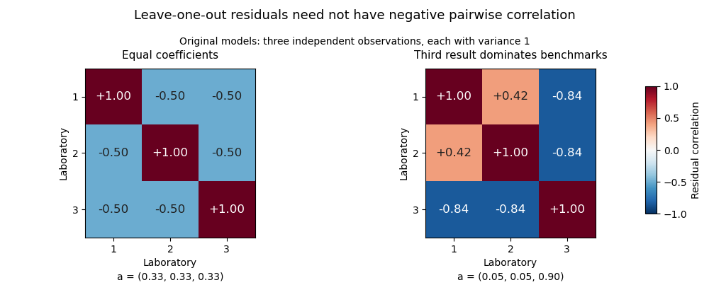
For positive inverse-variance weights $a_i=v_i^{-1}/W$, where $W={\sum }_k{v}_k^{-1}$, one has $a_i{v}_i=1/W$ and $S=1/W$. The off-diagonal expression becomesThus the leave-one-out inverse-variance weighted consensus has a special sign pattern under its independent known-variance assumptions.

The coefficients also impose a deterministic constraint,Consequently the residual covariance matrix is a singular matrix. Under the independent-observation model with every $v_i>0$, its matrix rank is $n-1$: the weighted centering matrix removes the common-level direction and the invertible diagonal matrix $M$ preserves that rank. For equal coefficients the constraint is simply ${\sum }_i{D}_i=0$.

These dependencies matter when evaluating several laboratories together. Products of single-residual probabilities generally do not describe joint events. A specified joint model or a set of appropriately chosen contrasts can represent the available information without treating redundant residuals as independent observations.

A leave-one-out inverse-variance weighted consensus applies an inverse-variance weighted mean to all laboratories except the one being assessed. Suppose their results $X_j$ are independent random variables with common expected value $\theta$ and known positive variances $u_j^2$. For laboratory $i$, defineUnder this model it is the best linear unbiased estimator of $\theta$ from the remaining results. The omitted observation does not determine its own leave-one-out interlaboratory consensus value.

The minimum-variance property follows directly from the Cauchy-Schwarz inequality. For any fixed coefficients $c_j$ satisfying ${\sum }_{j\ne i}{c}_j=1$, the linear unbiased estimator $T={\sum }_{j\ne i}{c}_j{X}_j$ hasEquality holds precisely for $c_j=u_j^{-2}/W_{-i}$. ThereforeThis is a comparison among linear unbiased estimators under the stated independent-error model; it requires no normal distribution assumption.

For an original example, assess a laboratory reporting $x_i=12$ with standard uncertainty $u_i=0.5$. The other laboratories report $(10,12,8)$ with respective standard uncertainties $(1,2,4)$, all in the same units. Their total precision is $W_{-i}=1+1/4+1/16=21/16$, givingThe held-out difference is $D_i=12/7\simeq 1.714$, withThe denominator includes the benchmark's uncertainty even though $X_i$ was excluded. This uncertainty-normalized difference and a proficiency-test z-score based on a predetermined assessment scale answer different questions.

Shared bias in an interlaboratory consensus changes the uncertainty model. Suppose instead $X_j=\theta +B+{\epsilon }_j$, where the common reference contribution $B$ has variance $u_B^2$ and the mutually independent residuals, independent also of $B$, have variances $s_j^2$. Coefficients summing to one preserve $B$ in the benchmark. Its variance is $u_B^2+\sum c_j^2{s}_j^2$, so the minimizing coefficients use $s_j^{-2}$, andUsing the full marginal uncertainties $\sqrt{u_B^2+s_j^2}$ as if they were independent changes the coefficients and loses the shared-reference structure. The propagation of uncertainty retains the covariance of dependent inputs.^[ref]

If the held-out laboratory shares the same $B$, that contribution cancels in $D_i$, while it remains in the benchmark's absolute measurement uncertainty. Precision of a difference and knowledge of an absolute value are distinct properties. Estimated, result-dependent uncertainties or additional correlations require analysis of the actual estimator; the fixed known-variance proof does not establish optimality for those cases.

A leading-edge radius fitting window is the chosen neighborhood of nose coordinates used in leading-edge radius estimation from sampled coordinates. It can be specified by coordinate bounds, arc length or a point-selection rule. The choice controls both how closely a local shape model applies and how strongly coordinate errors affect the inferred airfoil leading-edge radius.

Consider the original local model $x=A{y}^2+B{y}^4$, with known nose origin, exact $y$ coordinates and $A=1/(2r_0)>0$. A quadratic least squares fit with positive fixed weights givesThe quartic term therefore causes a deterministic coefficient error even with exact observations. For a dense, uniformly weighted window $-h\le y\le h$, the ratio of sums tends to $5h^2/7$. Expanding the window admits more of the omitted shape term.

Shrinking the window has a different cost. For unweighted observations with independent horizontal errors of common variance ${\sigma }_x^2$,At a fixed number of similarly distributed points, scaling every $y_i$ by one half multiplies this variance by sixteen. Very close points can have tiny horizontal displacements relative to the instrument's coordinate error. The window thus presents a concrete bias-variance tradeoff, not a rule that the smallest neighborhood is always best.

For stipulated $r_0=3$ mm and $B=10^7{\mathrm{m}}^{-3}$, the dense-window model gives fitted radii about 2.9682 mm at $h=0.5$ mm and 2.7362 mm at $h=1.5$ mm, before any noise is added. These are calculations on a specified quartic curve, not observed airfoil data. The broader window has less sensitivity to fixed coordinate noise but more quadratic-model bias.

A useful measurement report states the origin estimate, coordinate uncertainty, fitting model and exact window, then examines sensitivity to a few nearby windows. If both coordinates are uncertain or the nose location is fitted, the displayed variance formula no longer covers the complete estimation problem. A known analytic profile supplies an implementation check: the four-digit thickness envelope has the radius relation $r_{\mathrm{LE}}/c\simeq 1.1019{\eta }^2$.^[ref] That check cannot remove model error for an unrelated measured nose.