Topics (384k) Articles (398k) Users (410) Discussions (242) Comments (383) Files (13k) New article

Pairwise inclusion positivity requires every distinct pair of population units to have positive joint inclusion probability under the sampling design:For Horvitz-Thompson variance estimator, the probabilities must also be known, and individual inclusion probabilities must be positive. Each pair can then, at least in principle, contribute an observed product to a pair-expansion estimate. Positivity is not independence: need not equal .[ref]
Conservative variance estimation for sampling designs with zero pairwise inclusion probabilities by Peter M. Aronow and Cyrus Samii. Section 2, conditions for measurability; section 2.1, pair expansion
For simple random sampling of distinct labels from , . Consequently, gives pairwise positivity, whereas selecting exactly one label gives positive individual inclusion probabilities but zero probability of ever observing two distinct values together. This distinction separates unbiased total estimation from unbiased estimation of its sampling variance.
An original two-unit proof shows what information is missing. Sample one of two fixed values uniformly. The Horvitz-Thompson estimator is or , and its variance isAny estimator based only on the observed label and value has expected value of the form . Its mixed difference over is zero. The target's mixed difference is insteadNo such estimator can therefore be unbiased for this variance for every possible pair of values. Additional randomization internal to the estimator does not help: conditioning on the observed data still produces functions of this same separated form. This is an information limitation, not division by zero that can be repaired by assigning a convenient numerical convention.[ref]
Conservative variance estimation for sampling designs with zero pairwise inclusion probabilities by Peter M. Aronow and Cyrus Samii. Sections 1 and 2.2, impossible unbiased recovery of jointly unobservable cross-products
Strict positivity alone also does not guarantee useful precision. A very small produces a large inverse-probability multiplier on a rare observed pair. Designing a usable survey therefore requires attention to both observability and the resulting sampling variance.
In a rotating restricted three-body model, the Jacobi constant can be written , where is the effective potential. The zero-velocity surface bounds the accessible region: motion requires .
The surface is an energy constraint, not a physical wall or a trajectory. As changes, narrow connections can open near Lagrange points, permitting passage between previously separated regions. In a planar section these boundaries appear as zero-velocity curves. Actual passage still depends on the dynamics within the allowed region.
For observations in a known covariate order, the isotonic least squares estimator solvesIt is the orthogonal projection of the observation vector onto a closed convex cone of nondecreasing sequences. Strict convexity of the squared distance gives a unique estimate.
For data , the first pair violates monotonicity. Pooling it gives mean two, producing with squared error two. The pool adjacent violators algorithm repeatedly merges neighboring blocks whose means are out of order; the fitted value is constant at the block mean on each final block.
Positive observation weights replace squared error by and block means by weighted means. The order restriction regularizes the estimate without specifying a fixed polynomial form. The method requires the ordering to be meaningful; it does not discover an unknown covariate order from the response values.
A multifractal measure has different local scaling behavior at different points. For a measure on a metric space, a basic local exponent, when the limit exists, isIt describes how rapidly mass near shrinks with radius. The Hausdorff dimension of each level set gives a spectrum rather than a single dimension. The word does not require the measure to be invariant, although many examples come from invariant measures of dynamical systems.
For a concrete construction, repeatedly split into halves, giving relative mass to the left half and to the right, with . A level- interval with left choices has length and mass . Along a nested sequence with , its cylinder scaling exponent is . When , different digit frequencies produce different exponents. This is the mechanism by which uneven concentration of mass leads to several scaling laws.
The integrator reset settling time is the time required to reach a stated error band under the reset/readout sequence. It is not merely the switch's control propagation delay. The primary switch tutorial distinguishes switching time from complete-circuit settling.[ref]
MT-088: Analog Switches and Multiplexers Basics. pp11–13, Figures19–21
The integrator reset article derives an ideal residual , with . A focused extension includes an opening pedestal whose magnitude is at most . A conservative final-error bound isTo guarantee from this bound, require andwhen the logarithm is positive. This reset error budget with a persistent pedestal assigns separate parts of the tolerance to the residual and the opening event.
For stipulated , , and , the required duration is about . A tolerance of cannot be guaranteed by waiting longer under the same pedestal bound. Accidental cancellation of opposite-sign errors is not a worst-case guarantee.
Measure the output against a stated band at a reproducible delay after opening. Ringing, amplifier drive limits and prior overload can invalidate a single-exponential model; the device datasheet treats output-overload recovery separately.[ref]
ACF2101 Low Noise, Dual Switched Integrator datasheet. p10, Output Overload
The resulting acquisition exclusion is part of integrator reset dead time.A reset charge-injection pedestal is a step in the initial integrator output caused by charge transferred when the reset switch changes state. It can remain after an arbitrarily long preceding discharge. The integrator reset article distinguishes it from a decaying residual; the physical switched-integrator datasheet separately specifies charge-transfer errors.[ref]
ACF2101 Low Noise, Dual Switched Integrator datasheet. p3, Charge Transfer Errors
For an original example, let the net opening charge have magnitude on an integration capacitance of . The output step has magnitude . If interpreted as photodiode signal charge with constant responsivity , it would imitate of incident energy under the linear model. A positive step interpreted as signal would bias a true measurement by . The actual polarity depends on the circuit.
Repeated zero-input acquisitions at the same post-opening delay estimate the mean pedestal. Subtracting that mean does not remove reset pedestal variance. For a fixed capacitance, an opening-charge standard deviation of gives an output standard deviation of in the same stipulated model.
Varying the preceding reset duration helps distinguish residual discharge from a step created by opening. Gain, capacitance, signal level and readout delay must remain comparable. Adding capacitance can reduce the step per unit charge but also changes the signal conversion and the full circuit's settling behavior.
Integrator reset dead time is the interval during which incoming charge is excluded from the reported measurement because the integrator is resetting or not yet ready for acquisition. A switched-integrator implementation has distinct integration, hold and reset states; the historical datasheet shows those states and their timing.[ref]
ACF2101 Low Noise, Dual Switched Integrator datasheet. p9, Modes of Operation and Hold and Reset Switches, Figures3–4
For an original periodic schedule, acquire during the first of every cycle, reset for the next and exclude the final for settling. The duty cycle is . If short-pulse arrival phases are independent and uniform over that cycle, the expected captured fraction is .
That fraction does not apply to every pulse train. Pulses spaced by and arriving at phase are all missed in the ideal schedule. The same train at phase is entirely captured. The clock synchronization matters as much as the fraction of time spent acquiring.
A bench check compares accepted events with an independent pulse monitor while changing their phase relative to the reset command. State whether the excluded interval includes the switch delay, discharge interval, post-opening transient and readout recovery. A stable zero-input baseline alone cannot demonstrate that every pulse was accepted. The integrator reset settling time and a reset charge-injection pedestal concern readiness and initial conditions, while dead time concerns which signal arrivals contribute at all.
Input capacitance inferred from measured admittance is a parameter estimate from the quadrature component of a specified electrical port's response. In the parallel model of input capacitance, write its electrical admittance as with the convention. A small sinusoidal excitation and simultaneous input-current measurement giveBoth amplitude ratio and relative wave phase matter. The differential versus common-mode terminals and operating point conditions must be specified, as in the manufacturer's input-path diagrams.[ref]
MT-040: Op Amp Input Impedance by Analog Devices. Printed p. 1, Figure 1; printed p. 2, Op Amp Input Capacitance
For an original error calculation, suppose the amplitude ratio is exact but the measured current-to-voltage wave phase has offset . Then andThe phase calibration error in an admittance-based capacitance estimate can therefore mix a conductance term into the small capacitive estimate. For small , the leading error is , not a fixed percentage of .
Choose , , and . The true susceptance is only . A one-degree wave phase offset yields , an error of about , despite perfect amplitude readings. These are chosen port-model values, not measured device specifications.
A useful measurement repeats the estimate over frequency and excitation amplitude. A nearly constant fitted and a residual consistent with support the assumed model; they do not prove that all parasitic effects were removed. A known fixture admittance adds to a parallel port and must be subtracted or retained in the model. At very small susceptance, uncertainty in the relative wave phase can dominate, so a high DC input impedance alone is not evidence for a precise capacitance measurement.
A primary inner filter effect occurs when absorption within a sample weakens the excitation reaching the region from which fluorescence is observed. The measured intensity then depends on the excitation path as well as the emitting material. This differs from a secondary inner filter effect, which attenuates emitted light on its way to the detector.[ref]
Automatic Correction of Fluorescence Spectra for Primary and Secondary Inner-filter Effects (IFE) with Duetta by HORIBA. PDF p.1, Introduction and Fig. 1, excitation attenuation before the viewed region
Let be the incident photon rate and the absorbance from the entry face to a small observed region. The Beer-Lambert law gives the excitation reaching that region asFor and , the fractions reaching the region are approximately and . These absorbances describe the actual excitation path to the observed region, not automatically the entire sample-cell width.
A local model explains why more fluorescent material can even give less measured light. Suppose emitter concentration is , local fluorescence is linear in both and excitation, and path absorption is proportional to . Thenwith fixed positive and . The model rises to a maximum at and then falls, solely because the viewed region receives less excitation. With in compatible concentration units, raising from one to two changes the signal by . This is an illustrative small-region model, not a universal whole-cuvette response.
A useful diagnostic holds instrument settings fixed while recording both absorbance and fluorescence across a dilution or excitation-path-length series. A shorter path can reduce optical attenuation, but dilution can also change other sample properties. A declining signal alone therefore does not establish fluorescence quenching or a change of fluorescence quantum yield. JASCO distinguishes concentration quenching from this internal shielding mechanism.[ref]
A secondary inner filter effect occurs when emitted fluorescence is absorbed within the sample before reaching the detector. The absorption changes the collected signal and can distort its emission spectrum, especially when absorption differs strongly between emission wavelengths. It concerns the emitted-light path, whereas a primary inner filter effect concerns the excitation path.[ref]
Automatic Correction of Fluorescence Spectra for Primary and Secondary Inner-filter Effects (IFE) with Duetta by HORIBA. PDF p.1, secondary inner-filter effect and overlap of absorption/emission spectra
For a small emitting region followed by a purely attenuating detection path, let be the path absorbance at emission wavelength . The Beer-Lambert law gives the simple modelThe path geometry is part of this statement; a whole-cell absorbance must be scaled to the path actually traversed.
For a synthetic two-band example, suppose equal intrinsic signals of units face path absorbances and . The collected signals becomeTheir ratio is now , although the intrinsic ratio was one. A distorted band ratio can thus arise without a change in the relative emission initially produced.
Within this attenuation-only model, multiplying each observed band by recovers its intrinsic value. Real collection samples an extended volume, and scattering or absorption followed by re-emission can require a richer model. An absorbance-based correction is consequently meaningful only with its geometry and assumptions stated.[ref]
Automatic Correction of Fluorescence Spectra for Primary and Secondary Inner-filter Effects (IFE) with Duetta by HORIBA. PDF p.1, absorbance measurement and inner-filter correction discussion
A practical comparison measures an absorption spectrum along with fluorescence and repeats the measurement with a shorter detection path or suitable dilution. Record raw intensities as well as normalized spectra: normalizing peaks can hide a large loss of detected light. A fluorescence blank removes additive background under matched conditions, but does not by itself undo this wavelength-dependent attenuation.
The capacitive bridging complex-error bandwidth is the largest frequency over which a receiving port preserves the source phasor within a specified complex relative gain error. The criterion includes phase shift as well as amplitude. A large DC input impedance alone cannot establish this bandwidth when input capacitance matters. The manufacturer's input models explicitly include resistive and capacitive paths.[ref]
For the scalar impedance bridging with capacitive input model, assume a positive real source electrical resistance , receiver resistance , and input capacitance in parallel. Let be the unloaded source phasor. A voltage divider givesFor tolerance , the complex relative gain error isIts square is strictly increasing in , since its derivative is . Thus satisfying defines a continuous frequency interval starting at DC, whenever it is feasible. Rearranging givesThe DC error floor is . If , no frequency meets the tolerance; if , only DC does. The boxed positive bandwidth applies when .
For an original near-limit example, choose , and . Then and the DC error is about 0.9901 percent. A 1 percent full-complex tolerance leaves onlyAn amplitude-only 1 percent criterion, , instead allows about . The half-power (approximately ) signal bandwidth, relative to DC, is . These are three distinct specifications of this same ideal model.
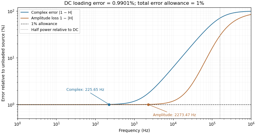
Complex-error, amplitude-error and half-power bandwidths can differ greatly
. Original 10 kilohm source, 1 megohm receiving resistance and 100 picofarad input-capacitance model. A one-percent complex error permits about 225.65 hertz; one-percent amplitude error permits about 2273.47 hertz. The half-power point relative to DC is about 160.75 kilohertz. Details.The square-root collapse of capacitive bridging bandwidth near the DC error floor follows by factoring the numerator:For fixed and ,This asymptotic equivalence explains the sharp loss of usable bandwidth when the resistive divider has already consumed nearly all the error allowance. Increasing or reducing changes that floor; reducing only rescales a feasible bandwidth but cannot remove infeasibility at DC.
The criterion also controls a complete waveform. Suppose a source waveform is both a square-integrable function and a bandlimited function, with spectrum supported where . For the corresponding zero-state response , the Fourier transform of is . The Plancherel theorem, or the norm bound for a Fourier multiplier on L2, givesHere the Fourier transform uses the frequency-in-hertz convention, so the displayed Plancherel theorem has no extra normalization factor. This bound includes waveform changes caused by phase. It applies to the zero-state response of the stated frequency response. Any additional homogeneous solution from initially stored energy contributes its own error.
A bench check therefore needs both amplitude ratio and phase shift, with probe and cable capacitance included in the port model. Magnitude-only observations determine without determining . The formula describes this chosen passive input network; additional amplifier dynamics require their own transfer function.
Iduronate is the conjugate base of iduronic acid, formed when its carboxyl group loses a proton. Starting from neutral , proton loss gives the free-monomer molecular formula . The usual biological discussion concerns the L-iduronate series.[ref]
Ionization and epimerization are different operations. Removing the acidic proton changes electric charge without changing the carbon stereochemistry. Conversely, heparosan-N-sulfate-glucuronate 5-epimerase converts D-glucuronate residues into L-iduronate residues by changing carbon-5 configuration within a polymer.[ref]
Charge accounting makes the distinction quantitative. A solution containing of singly charged iduronate anions requires one millimole of monovalent positive counterions for electrical neutrality, if no other charged species contribute. That statement concerns charge balance, not a specification of which salt was prepared. In a polysaccharide, the iduronate name instead refers to a linked residue; its atom inventory cannot be substituted unchanged for a free monomer's formula.
Idler bearing load sharing determines how an idler support reaction is divided among the shaft's supporting bearing elements. Zero net torque on an ideal steady idler gear does not remove its mesh-induced transverse force. The bearing loads additionally depend on axial positions and the supported-shaft arrangement. Manufacturer guidance separates a radial load between two bearings from an overhung load and treats gear loads as applications of those cases.[ref]
Model the shaft as a simply supported beam with supports A and B at axial coordinates and . Let a gear resultant act upward at , and take upward reactions as positive. Static equilibrium requiressoFor a200N mesh resultant at between supports100mm apart, the downward reactions are120N and80N. Equal division occurs only for the centered load in this symmetric ideal support model.
For overhung idler loading at with the same support span and resultant, and . The farther support's force reverses direction, and the nearer bearing carries more than the applied resultant. This does not violate force balance: . If a particular support cannot provide the required reaction direction, the assumed support model must change.
For loads in two transverse directions, solve each component balance before forming the resultant at each bearing. Helical gears add gear axial force; allocating that thrust requires the actual bearing constraints and cannot be inferred from the transverse lever rule. More than two effective supports generally require deformation compatibility as well as equilibrium. These calculations estimate support forces, rather than directly determining bearing life or internal rolling-element contact loads.
Timing spread and gain-offset estimator covariance describes how delivery durations affect both precision and correlation when a known volume calibrates an integrated volumetric flow rate sensor. In the model , assume and durations are known and independent volume errors have common variance . Define .
The least squares slope estimates offset , while the intercept divided by estimates gain . Their covariance isThe negative covariance reflects a tradeoff: a larger fitted offset can be compensated by a smaller gain while preserving responses near the middle of the observed durations.
For an original design with L, durations 1 and 6 s, and L, the standard uncertainties are approximately 0.00283 L/s for offset and 0.00406 for gain. Their correlation is about . Moving the second duration to 2 s, with everything else stipulated unchanged, makes the offset uncertainty five times larger. Wider duration spread supplies more leverage for separating slope from intercept within this model.
Prediction shows why the covariance matters. For a new duration , the fitted mean response is , withAt the midpoint 3.5 s in the example, its standard uncertainty is L. Incorrectly dropping the gain-offset covariance would give about 0.0157 L. This is uncertainty of the fitted mean; an independent future observation adds its own error variance.
Centering time at makes the fitted midpoint response and slope uncorrelated under the stated equal-variance model. Transforming back to physical gain restores the covariance, so a change of coordinates does not remove shared uncertainty. The GUM explicitly retains such covariance terms in propagation.[ref]
Guide to the expression of uncertainty in measurement by JCGM. §5.2.2, equation 13, correlated-input propagation
Reference-volume uncertainty, uncertain timing and nonlinear volumetric flow rate response require additional terms beyond this original regression calculation.An ideal in a commutative ring is finitely generated if there are such thatThe generators need not generate as an additive group; arbitrary ring coefficients are allowed. The zero ideal is generated by zero, or by the empty list under that convention.
For example, in : both generators are divisible by two, while gives the reverse inclusion. In , the ideal consists of polynomials with zero constant term.
Finite generation is not automatic in every ring. In , the ideal of all polynomials with zero constant term is not finitely generated. Any finite list involves only finitely many variables; setting those variables to zero kills the generated ideal but leaves an unused variable nonzero. A Noetherian ring is exactly a commutative ring in which every ideal is finitely generated.
A hyperprior is a prior distribution assigned to a hyperparameter that controls another prior distribution. In a hierarchical Bayesian model, this makes uncertainty about the prior's parameters part of the joint probability model, rather than replacing those parameters by fixed numbers.[ref]
Stan User's Guide by Stan Development Team. Version2.37, Regression Models, Hierarchical priors
For data , a model parameter and a hyperparameter , a common factorization isHere supplies the likelihood function, is the conditional prior distribution, and is the hyperprior. After observing , Bayesian inference gives a joint posterior distribution. The marginal posterior of averages over the updated hyperparameter distribution:For discrete hyperparameters, the integral is replaced by a sum.
An exact example makes the averaging visible. Let be a success probability and choose a two-point hyperprior,Both conditional beta distributions have expectation , but they concentrate differently around it. Now observe two successes that are independent conditional on , each with a Bernoulli distribution. Their conditional probability is . Integrating against the two possible priors givesThus the data also update the hyperparameter:The conditional posterior distributions of are respectively and . Their posterior mixture has meanThis is an original illustrative probability model, rather than data or a numerical example from the guide.
Fixing at its prior mean would instead produce after the same observations, with posterior mean . Averaging the hyperparameter first has changed the model; it does not reproduce averaging the conditional posteriors with their updated probabilities. A hyperprior therefore adds a specified layer of uncertainty, while its own choice remains part of the assumptions of the hierarchical Bayesian model.
Water-denominator effects in nail concentration measurements occur when a concentration changes because the amount of retained water changes the sample mass used for normalization. This can happen without any change in the amount of the measured substance. The denominator is part of the reported observable.
For an original inventory model, let be the retained marker amount, structural mass and water mass. Define the water fraction of wet material as . Concentrations on the two stated bases obeyAt fixed and , increasing hydration lowers while leaving unchanged. The structural basis here is a model-defined material amount; an actual drying procedure must establish what it retains before being equated with .
For stipulated ng and mg, increasing from 2 to 5 mg changes the wet-basis concentration from to ng/mg, a 20% decrease. Both concentrations correspond to 10 ng/mg on the structural basis. Comparing the wet values alone would falsely suggest a marker loss if unchanged hydration were assumed.
The relation also affects pooled samples. Take two clippings with equal structural mass 10 mg and equal marker amount 100 ng, but water amounts 0 and 10 mg. Their wet-basis concentrations are 10 and 5 ng/mg. Pooling gives ng/mg, rather than the unweighted average 7.5. Mass-normalized temporal kernels for nail clippings must therefore use the same mass basis as the constituent concentrations.
A further assay factor can change the numerator as well. If a fraction of the retained marker is recovered, the measured quantity is . Correcting water content cannot by itself establish or prove that stayed constant. An original comparison should independently track conditioning, sample mass and recovery before attributing a concentration difference to changed incorporation.
A primary ellipsometry experiment observed the complex refractive index of fingernails during hydration and dehydration, relating the response to water associated with keratin.[ref]
Hydration dynamics of human fingernails: An ellipsometric study by B. Schulz and others. Abstract, changing optical response and water interpretation
This supports treating hydration as a material-state variable. The denominator equations follow from conservation of mass; the optical experiment does not directly measure marker retention or matrix production.Hot-wire spatial averaging is the loss or alteration of small-scale flow information because a heated sensing wire has finite spatial extent. Even a perfectly fast electronic readout observes a spatially distributed heat-transfer response. The manufacturer's practical guide relates spatial resolution to wire dimensions, flow and instrument frequency response.[ref]
An original small-perturbation model treats the inferred velocity fluctuation as a uniform line average over wire length . With measuring distance along the wire,For a spatial sinusoid , direct integration givesThis is a sinc function transfer factor. It follows from the stipulated uniform weighting and local linearity; a real wire's nonuniform temperature and nonlinear heat transfer require a more detailed spatial kernel.
For spatial wavelength , a fluctuation with has amplitude factor about and variance or power factor . At , the factors are and . At , one complete sinusoidal cycle lies along the wire and its line average is exactly zero. Raising the sample rate cannot restore a component that this spatial average has canceled.
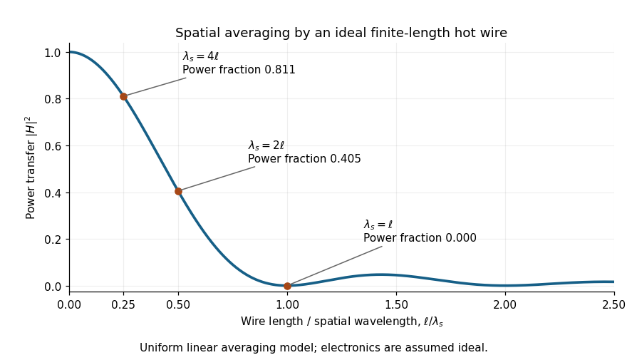
For a wire, these illustrative wavelengths are , and . The result depends on the component of the spatial wavevector along the wire, rather than only on a temporal frequency. Orientation-dependent spatial filtering by a hot wire matters because a moving three-dimensional structure can have different projections along the wire and the mean flow. Under a frozen-advection model, temporal frequency obeys ; substituting into the wire-length factor requires an additional alignment assumption.
Spatial and temporal filters can both reduce measured fluctuation variance. In this single-sinusoid model, the measured variance is times the true variance even with noiseless electronics. A correction obtained by dividing by becomes unstable near its zeros, amplifying measurement noise without recovering independently lost information.
A proposed test compares probes of different active lengths in the same statistically repeatable flow, after separate steady calibrations and matched electronic filtering. Record wire orientation, support geometry, ambient temperature and traverse location; compare fluctuation spectra as well as mean velocity. A difference that tracks wire length supports a spatial-filtering interpretation, but changed thermal response or probe disturbance must also be checked. The observation establishes the filtered response of the actual apparatus over its characterized range, not an unqualified point measurement at every turbulent scale.
The single-draw variance identifiability obstruction is the inability, for an unrestricted finite population, to construct a universally design-unbiased estimate of a total estimator's variance from just one observed unit. The estimator can estimate the total unbiasedly while the required cross-products for estimating its sampling variance are never jointly observed. This is an obstruction to the stated one-draw estimation problem, not a claim that a parameter can never be identified from repeated independent samples.
An original two-unit proof makes the distinction exact. Sample label or2 with equal probability and observe only . The Horvitz-Thompson estimator of the finite population total is . Its expectation is , and its design variance isSuppose a proposed variance estimate returns after observing unit1 and after observing unit2. Unbiasedness for every pair would requireThe left side is additive in the two unknown values, while the right side contains an unobserved product.
To prove impossibility without smoothness assumptions, evaluate both sides at . Every additive function has rectangular contrast . The required variance has contrast . The contradiction rules out such an unbiased estimator. Independent auxiliary randomization does not help: averaging it out merely replaces each by another function of the same single observed value.
Here the individual inclusion probabilities are positive, but the joint inclusion probability for distinct units is zero. The usual Horvitz-Thompson variance estimator needs pairwise inclusion positivity to turn sample cross-products into unbiased population cross-product estimates. The primary analysis of zero pairwise probabilities identifies precisely these missing terms.[ref]
Conservative variance estimation for sampling designs with zero pairwise inclusion probabilities by Peter M. Aronow and Cyrus Samii. §2.1, pair-expansion variance estimator; §2.2 and Proposition1, missing products under zero pairwise probabilities
Extra information can change the problem: observing suitable pairs, imposing a justified population relation, or accepting a model-based or conservative estimate uses assumptions absent from the proof. Observing one value also does not prevent writing a biased variance estimate. What fails is a single-draw unbiased estimator valid for every unrestricted population, even though the total estimator itself remains unbiased.
Pinned article: Introduction to the OurBigBook Project
Welcome to the OurBigBook Project! Our goal is to create the perfect publishing platform for STEM subjects, and get university-level students to write the best free STEM tutorials ever.
Everyone is welcome to create an account and play with the site: ourbigbook.com/go/register. We belive that students themselves can write amazing tutorials, but teachers are welcome too. You can write about anything you want, it doesn't have to be STEM or even educational. Silly test content is very welcome and you won't be penalized in any way. Just keep it legal!
Intro to OurBigBook
. Source. We have two killer features:
- topics: topics group articles by different users with the same title, e.g. here is the topic for the "Fundamental Theorem of Calculus" ourbigbook.com/go/topic/fundamental-theorem-of-calculusArticles of different users are sorted by upvote within each article page. This feature is a bit like:
- a Wikipedia where each user can have their own version of each article
- a Q&A website like Stack Overflow, where multiple people can give their views on a given topic, and the best ones are sorted by upvote. Except you don't need to wait for someone to ask first, and any topic goes, no matter how narrow or broad
This feature makes it possible for readers to find better explanations of any topic created by other writers. And it allows writers to create an explanation in a place that readers might actually find it.
Figure 1. Screenshot of the "Derivative" topic page. View it live at: ourbigbook.com/go/topic/derivativeVideo 2. OurBigBook Web topics demo. Source. - local editing: you can store all your personal knowledge base content locally in a plaintext markup format that can be edited locally and published either:This way you can be sure that even if OurBigBook.com were to go down one day (which we have no plans to do as it is quite cheap to host!), your content will still be perfectly readable as a static site.
- to OurBigBook.com to get awesome multi-user features like topics and likes
- as HTML files to a static website, which you can host yourself for free on many external providers like GitHub Pages, and remain in full control

Figure 2. You can publish local OurBigBook lightweight markup files to either OurBigBook.com or as a static website.
Figure 3. Visual Studio Code extension installation.
Figure 5. . You can also edit articles on the Web editor without installing anything locally. Video 3. Edit locally and publish demo. Source. This shows editing OurBigBook Markup and publishing it using the Visual Studio Code extension. 
- Infinitely deep tables of contents:




All our software is open source and hosted at: github.com/ourbigbook/ourbigbook
Further documentation can be found at: docs.ourbigbook.com
Feel free to reach our to us for any help or suggestions: docs.ourbigbook.com/#contact