Drift-aware homogeneity analysis estimates material variation while accounting for time-dependent changes in the measurement system. Its purpose is to prevent instrumental drift from being assigned to differences between containers in a homogeneity study with replicated test portions. The recorded order is part of the experimental data.

A simple measurement model iswith container contribution $b_i$, linear drift rate $\gamma$ and residual $e_{ij}$. A linear regression can treat container differences as fixed effects; a random effect formulation instead models a between-container variance. Either approach must distinguish the time term from the container terms. Homogeneity-study time-term identifiability depends on the actual sampling schedule.

An original noiseless example uses A at times 0 and 5 with readings 100 and 105, B at 1 and 4 with readings 103 and 106, and C at 2 and 3 with readings 101 and 102. Each within-container difference divided by its time separation gives drift rate one. Subtracting that rate times observation time yields A readings 100, B readings 102 and C readings 99. The adjustment retains the true stipulated container differences instead of forcing all means to coincide.

With noise present, the rate is uncertain. Substituting a fitted rate and then analyzing the adjusted observations as if that rate were known omits its uncertainty and induced covariance. For example, six observations with an intercept, two independent container indicators and one time coefficient leave only two residual statistical degrees of freedom when the design has full rank. A more elaborate drift curve consumes information and may explain away genuine material differences.

Randomized order and control observations help diagnose the model. The IUPAC protocol requires randomized analysis of duplicate portions and checking trends or other suspect data features.^[ref] Separately, NIST's dimensional-comparison designs deliberately balance some drift contributions through observation order.^[ref]

Plot residuals against time and container, retain independent controls, and state how the time dependence was chosen. A fitted linear term does not establish that all drift is linear. If time and container effects cannot be distinguished, the study needs additional information or a better design rather than an unjustifiably precise homogeneity estimate.

The lateral habenula is the lateral division of the habenula, an epithalamic nuclear complex. Its circuits participate in linking information about outcomes and aversive events to other brain systems. It is an anatomical structure containing varied neuronal activity, rather than a uniform label for every negative emotion.^[ref]

In a rhesus-monkey eye-movement task, many lateral-habenular neurons responded more strongly to targets predicting no reward and less strongly to rewarded targets. Reversing which location earned reward reversed these responses. That control distinguishes outcome association from an unchanging preference for a screen location. Habenular excitation preceded dopamine-neuron inhibition on unrewarded trials, and weak stimulation inhibited dopamine-neuron activity.^[ref]

Temporal organization is another experimentally important property. A 2018 study of rat and mouse models examined increased burst firing and its suppression by ketamine. Pharmacology and modeling implicated NMDA receptors and T-type calcium channels, and controlled current changes could switch recorded neurons between bursting and tonic firing modes.^[ref]

An invented comparison makes the distinction clear: ten evenly spaced spikes and two tight bursts of five spikes over the same observation period have the same total count and mean rate, but different timing. A mean firing rate alone can miss the property a burst experiment tests.

The studies support specific circuit and cellular hypotheses. They do not establish a direct monosynaptic inhibitory connection from the stimulation result alone, or show that rodent behavioral assays explain every aspect of human depression or ketamine action. Anatomy, response polarity and firing pattern answer related but different questions.

The medial habenula is the medial division of the habenula, a nuclear complex of the epithalamus. It participates in a circuit projecting to the interpeduncular nucleus. The medial habenula and lateral habenula are neighboring anatomical divisions with different circuitry; results from one should not automatically be assigned to the other.^[ref]

A motivating experiment tested an inhibitory contribution to nicotine intake. Christie D. Fowler and colleagues found increased nicotine intake in mice lacking the α5 nicotinic acetylcholine receptor subunit. Re-expression of that subunit in the medial habenula rescued the altered intake phenotype; knockdown in the medial habenula of rats reproduced increased intake. The work distinguished nicotine's rewarding effects from an inhibitory effect appearing at higher tested doses.^[ref]

The rescue is particularly informative. A whole-animal mutation can alter many tissues and developmental processes. Restoring the relevant component in a specified region tests whether that regional circuit can account for an important part of the phenotype. Conversely, the comparison does not show that every medial habenula neuron has the same function or that the entire region is merely a nicotine-detector. The measured intake change is a result in specified rodent preparations, not a direct measurement of human smoking behavior or a clinical intervention.

A complete graph invariant is a graph invariant whose value determines a graph up to graph isomorphism. For graphs in a specified class, completeness meansAn ordinary invariant only requires the forward preservation statement $G\cong H\Rightarrow I(G)=I(H)$. Completeness adds the converse: equal values must exclude graph non-isomorphism.

A direct construction proves that complete invariants exist for finite undirected simple graphs. For an $n$-vertex graph, label its vertices $1,\dots ,n$ and list the entries above the diagonal of its adjacency matrix in the fixed order $(1,2),(1,3),\dots ,(n-1,n)$. This gives a binary string. Repeat for every labeling and choose the least string in lexicographic order. Define $I(G)$ to be the pair consisting of $n$ and this least string. Including $n$ distinguishes graphs whose edge string is empty but whose vertex counts differ.

Relabeling a graph permutes the same collection of candidate strings, so isomorphic graphs have the same minimum. Conversely, if two minima and vertex counts agree, some labeling of each graph gives exactly the same adjacency entries. Matching vertices with those labels is an isomorphism. This proves both directions, without assuming that the construction is computationally fast.

For an original three-vertex example, a path's possible strings are $011$, $101$ and $110$ in the order $(12,13,23)$. Its invariant is $(3,011)$. A triangle instead gives $(3,111)$. The difference certifies non-isomorphism. For larger graphs the naive construction may examine $n!$ labelings, so mathematical completeness alone supplies no practical speed guarantee.

Canonical graph labeling produces a standardized labeled representative and is closely connected to this construction. The authors of nauty and Traces identify canonical-label production as one of their programs' tasks.^[ref] A particular program's chosen representative need not be the lexicographically least string used in this illustrative definition; comparisons must use the same canonization convention.

Vertex count, edge count and degree sequence are useful inexpensive invariants but are not complete. The example in graph non-isomorphism gives equal values for all three while connectedness differs. Completeness concerns the information retained, separately from the effort required to compute it.

A granulosa-lutein cell is a granulosa cell that has undergone luteinization, acquiring the differentiated endocrine state associated with the corpus luteum. It can produce progesterone while retaining experimentally measurable regulation of other steroid pathways. The label identifies origin and cell state, rather than a separate oocyte or an entire ovarian follicle.

In a 1991 human-cell experiment, luteinized granulosa preparations were cultured for48hours with or without human chorionic gonadotropin or follicle-stimulating hormone. The investigators separately measured steroid production and aromatase activity. This demonstrated several regulated biochemical outputs in the luteinized preparation.^[ref]

A later assay study addressed an important measurement problem: estradiol accumulation depends on available androgen substrate as well as aromatase. After a stimulation period, investigators washed the cultured granulosa-lutein cells and supplied testosterone for a separate short assay. Changing when substrate was supplied made the test of follicle-stimulating hormone responsiveness more interpretable.^[ref]

A result from these cells should therefore identify the culture interval, stimulation and assay substrate. It cannot automatically describe the behavior of an unmodified granulosa cell at every stage of follicular development.

In a graded ring $R={⨁}_{d\ge 0}{R}_d$, a homogeneous element of degree $d$ is an element of the component $R_d$. Every ring element is a finite sum of homogeneous components. A nonzero homogeneous element has a unique degree because the sum is direct; zero belongs to every component and usually has no unique assigned degree.

In $k[x,y]$ with total-degree grading, $x^2+3xy-y^2$ is homogeneous of degree two, although it has three terms. The element $x^2+y$ is not homogeneous: its nonzero components lie in degrees two and one. The grading rule gives $R_d{R}_e\subseteq R_{d+e}$, so a nonzero product of homogeneous elements has degree $d+e$.

Grading depends on the declared convention. Assigning weight two to $x$ and weight one to $y$ makes $x+y^2$ homogeneous of weighted degree two. Homogeneity organizes computations in graded modules and the equations used in projective geometry.

Curvature bias in Gouy-phase measurements occurs when a spatially varying wavefront-curvature wave phase is mistaken for the axial Gouy phase in an interferometric comparison. For a fundamental Gaussian beam with time convention $e^{-i\omega t}$, the signal wave phase containsA curved reference contributes its own quadratic wave phase. After subtracting common axial path terms, the measured relative wave phase isThus a phase-retrieval algorithm can work exactly while the subsequent physical interpretation is biased. The Gaussian confinement wave phase and its arctangent dependence are derived in the primary theoretical treatment.^[ref]

For an original example with a planar reference and stable path wave phase, let $R_s(z)=z[1+(z_R/z{)}^2]$ and $z_R=k{w}_0^2/2$. At $z=z_R$ and fixed detector radius $r=w_0$, the curvature term is 0.5 radians. The true axial contribution is $-\pi /4$, whereas that off-axis pixel gives $-\pi /4+0.5\simeq -0.2854$ radians. At $z=-z_R$ the curvature term reverses. Comparing those two axial planes at this fixed radius gives a wave phase change $-\pi /2+1$, differing from the axial Gouy change by one radian.

The effect is observable even where the signal is appreciable: at $z=z_R$, $r=w_0$ is inside the plane's Gaussian radius $\sqrt{2}{w}_0$. Avoiding only dim pixels does not remove curvature bias.

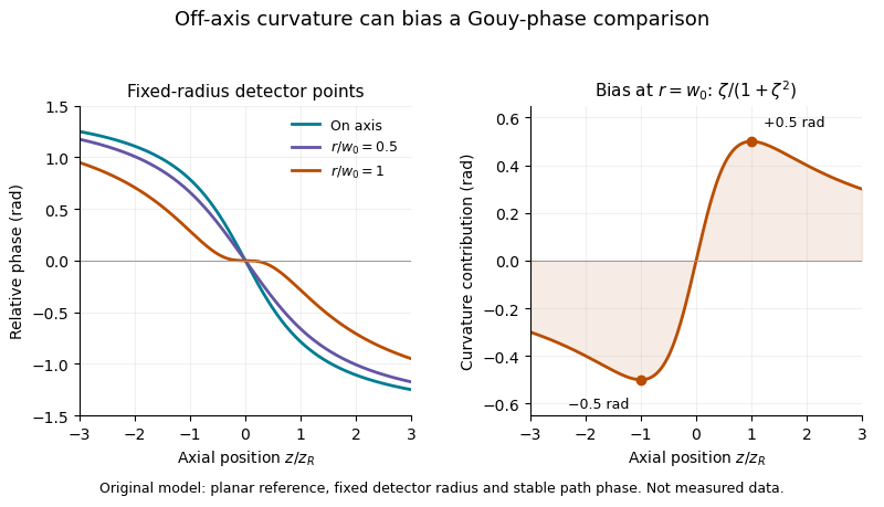
A useful measurement fits the spatial quadratic wave phase, identifies the beam center and reference curvature, and extrapolates the relative wave phase to the axis. Tilt, decentering and path drift require their own terms; averaging several pixel phases is not automatically equivalent to measuring the on-axis wave phase. Phase unwrapping can be required before fitting a wave phase profile.

The primary 2023 Bessel-Gaussian experiment documents focusing optics and a rail-mounted camera in its interferometer.^[ref] It motivates tracking both propagation position and wavefront geometry, but its structured-mode observations must not be silently reclassified as measurements of the illustrative fundamental-Gaussian model above.

The nerve lemma identifies a space with the geometric realization of the nerve of a sufficiently well-behaved good cover, up to homotopy equivalence. A standard version assumes a paracompact Hausdorff space with an open good cover: every nonempty finite intersection is contractible. The nerve has one vertex per covering set and one simplex per nonempty finite intersection.^[ref]

Cover a circle by three open arcs chosen so each pair overlaps in an interval and there is no triple intersection. The nerve has three vertices and three edges, but no filled triangle, so it has the homotopy type of a circle. Filling in that triangle would incorrectly make it contractible. The example shows why one must track all intersections, rather than only whether the individual covering sets are contractible.

N-sulfation of glucosamine attaches a sulfur-containing group at the nitrogen of an eligible glucosamine residue. In heparan sulfate biosynthesis, this changes nitrogen substitution within a polysaccharide; it does not add a new sugar residue or change which carbon atoms form the backbone.

The enzyme heparan sulfate glucosamine N-sulfotransferase transfers a group from the activated donor PAPS to polymer-associated glucosamine. Its official reaction produces the N-sulfated sugar position and adenosine3′,5′-bisphosphate. This specifies both the donor and the modified atom, rather than treating free inorganic sulfate as a complete account of the reaction.^[ref]

An N-acetylated position must first lose its acetyl group before that nitrogen can undergo the corresponding N-sulfation. Nitrogen substitution also matters downstream: heparosan-N-sulfate-glucuronate 5-epimerase recognizes particular neighboring N-sulfated arrangements when changing glucuronate into iduronate.^[ref]

For an original ideal stoichiometric example, modifying 12 eligible nitrogen positions consumes 12 PAPS donor molecules. A chain segment that initially contained 40 sugar residues still contains 40 afterward. Counting sulfur incorporation and counting chain extension therefore measure different processes; counting total sulfur also cannot locate which nitrogen or oxygen positions were modified.

A global maximizer of $f:X\to \mathbb{R}$ is a point $x_{\ast }\in X$ satisfying $f(x_{\ast })\ge f(x)$ for every $x\in X$. The global maximum is the attained value $f(x_{\ast })$; argmax collects all points attaining that value:The set can be empty or contain many points. For $f(x)=\cos x$ on the real line, the global maximum is one and the global maximizers are $2\pi k$, $k\in \mathbb{Z}$. No single representative is specified by the optimization problem.

A stationary point is a different kind of condition. For a differentiable function on an open real interval, an interior global maximizer has zero derivative, but the converse fails: $f(x)=x^3$ has zero derivative at zero without a local maximum. A boundary global maximizer need not have zero derivative either; $f(x)=x$ on $[0,1]$ attains its largest value at the right endpoint.

The extreme value theorem supplies a useful sufficient existence condition: a continuous function on a nonempty compact set attains its maximum. Compactness is sufficient, rather than necessary; the cosine example attains a global maximum on the noncompact real line.

The molar Gibbs free energy is the Gibbs free energy per amount of substance, $G_m=G/n$, with units $\mathrm{J}\mathrm{mo}{\mathrm{l}}^{-1}$. For a homogeneous pure substance, extensivity gives $G=n\mu$, so $G_m$ equals its chemical potential $\mu$.

For a mixture, $G/n$ is an average over the components; the separate chemical potentials are the partial derivatives ${\mu }_i=(\partial G/\partial n_i{)}_{T,p,n_{j\ne i}}$. Equality of a component's chemical potential in two phases is a condition for phase equilibrium. This explains why comparing molar free energies predicts which phase of a pure substance is stable at specified temperature and pressure.

A truncated geometric distribution is obtained by conditioning a geometric random variable to lie in a specified finite range. For the trials-until-success convention $\mathrm{Pr}(T=k)=p(1-p{)}^{k-1}$ and an integer $m\ge 1$,The denominator is the probability of at least one success in the first $m$ independent Bernoulli trials. It renormalizes the retained probabilities.

For $p=1/2$ and $m=3$, the conditional probabilities are $4/7,2/7,1/7$. This differs from censoring or capping at $m$: the variable $\min (T,3)$ has probabilities $1/2,1/4,1/4$, because all later successes accumulate at three. Specifying conditioning rather than capping is essential in models of bounded retries. As $m\to \infty$, the conditioned probabilities tend to the original geometric distribution.

Gear friction work per engagement is the mechanical energy dissipated by sliding during one tooth pair's active engagement. It is the time integral of that pair's gear sliding-friction loss:The result has units of joules, whereas instantaneous loss has units of watts. It excludes other gearbox losses such as support friction. Manufacturer efficiency guidance distinguishes meshing and support losses and emphasizes their dependence on operating conditions.^[ref]

For a fixed-axis external spur gear pair, let signed contact coordinate $s$ run from $-L_a$ to $L_r$ through the gear pitch point. Gear sliding velocity has magnitude $(|{\omega }_1|+|{\omega }_2|)|s|$. At constant shaft speeds, gear base-roll speed gives $ds/dt=u_b>0$ in this chosen direction. If $\mu$ and the force carried by this pair are constant,With hypothetical $\mu =0.05$, $F_n=100\mathrm{N}$, angular-speed sum75rad/s, $L_a=5.0586\mathrm{mm}$, $L_r=4.5960\mathrm{mm}$ and $u_b=0.93969m/s$, this gives about9.32mJ. Doubling both shaft speeds doubles instantaneous power but halves gear contact duration, leaving this idealized work per engagement unchanged. Real friction and load can themselves change with speed.

Gear tooth load sharing is essential when several pairs engage simultaneously. A constant total mesh load is not a constant full load on each active pair. If identical pair events recur at gear mesh frequency $f_m$, averaging their correctly modeled losses over many events gives $\overline{P}=f_m{E}_f$. The event's force history must already include load sharing; assigning the whole mesh load independently to every overlapping pair would overcount transmitted load and loss.

A gear inspection coverage audit records which parts of a tooth surface were eligible for observation, which were excluded and why. It accompanies a gear pitting area fraction or gear inspection common-region comparison so that a numerical damage statistic can be interpreted against the area actually inspected.

A useful record retains the original image, gear pitting inspection mask, surface-coordinate map from image registration, represented pixel areas and exclusion reasons. Shadow, occlusion and an out-of-frame edge are different from a visible region classified as intact. An audit also distinguishes changes in viewing coverage from changes in the image segmentation rule.

An original calculation shows how missing area limits interpretation. Let inspected fraction $c=A_{\mathrm{seen}}/A_{\mathrm{target}}$ and observed pitting fraction ${\varphi }_{\mathrm{seen}}$ both refer to the same target surface. If unseen area has unknown pitting fraction $0\le {\varphi }_{\mathrm{unseen}}\le 1$, thenso the gear inspection missing-area bound isAt $c=0.8$ and ${\varphi }_{\mathrm{seen}}=0.02$, the whole-target fraction lies between $0.016$ and $0.216$ without further information. This is a deterministic range over missing data, not a statistical confidence interval. A small observed fraction does not alone establish a small whole-target fraction.

For repeated inspections, record areas visible only initially, only later and at both times. A common-region result can be valid for its intersection while becoming less representative of the full target if a damaged edge is systematically lost. Increasing pixel count inside the retained region does not recover information about the missing region.

The primary NASA gear-endurance study connected inspection history to vibration and oil-debris observations, illustrating the importance of tying a damage interpretation to physical inspection rather than a signal label alone.^[ref] The audit and bound above specify an explicit measurement convention; they do not assert that the historical study used this digital-mask procedure.

A gear marking-layer gap threshold is an effective separation below which a stated marking process produces a visible transfer or removal of material. It is a model of the observation in a gear contact marking test, rather than a universal thickness or a material constant. Layer thickness, pressure, rolling history and the marking material can all matter; a visible gear contact pattern does not directly give local operating pressure.

For an original idealization, let the unloaded separation across a face beand stipulate a visible mark where $g(z)\le h$. Here $h$ is the effective threshold, $g_0$ the minimum gap and $a>0$ its slope magnitude. For a centered pattern on face width $b$, the predicted marked width isChoose $b=20\mathrm{mm}$, $g_0=0.5\mu \mathrm{m}$ and $a=0.4\mu m/mm$. Thresholds $h=1.5$ and $2.5\mu \mathrm{m}$ give marked widths $5$ and $10\mathrm{mm}$. The geometry has not changed; the observation threshold has.

Away from the onset and saturation corners,Here a threshold change $0.2\mu \mathrm{m}$ changes the indicated width by $1\mathrm{mm}$. In the shallow-gap limit, small changes of the marking process can therefore cause conspicuous changes in the visible pattern.

A controlled comparison should hold the coating method, applied torque and number/direction of roll-throughs fixed, then vary one geometric setting. A separate fixture with known separations can test whether a proposed threshold model describes the marking process, without treating nominal coating thickness as an exact gap measurement.

Manufacturer contact guidance describes patterns as evidence about assembled tooth surfaces, and the historical rating standard limits the load information inferred from a bearing pattern.^[ref][ref] The threshold equation is a deliberately specified illustrative model; actual deformation and transfer behavior need validation before converting a mark into a quantitative gap or gear face load distribution.

Gear base-roll speed $u_b$ is the rate at which base-circle rolling advances an ideal involute contact along the gear line of action. For a fixed-axis external pair at constant speed,The equality follows from the tooth-count speed ratio and compatible base pitches. It describes the rate of change of contact position along a geometric line, rather than the gear sliding velocity between material points on the flanks. Base circles and their common tangent define this geometry.^[ref]

For standard module2 gears with20 and40 teeth at20degree reference angle, base radii are $r_{b1}=20\cos 20{}^{\circ }\mathrm{mm}$ and $r_{b2}=40\cos 20{}^{\circ }\mathrm{mm}$. Signed angular velocities ${\omega }_1=50rad/s$ and ${\omega }_2=-25rad/s$ give the same $u_b\approx 0.93969m/s$. The first gear's reference-circle tangential speed is1m/s, so base-roll and pitch-circle speeds are distinct.

In one tooth-entry interval, the base circle advances one gear base pitch:With $f_m\approx 159.155\mathrm{Hz}$, the example advances5.90426mm per entry. An active contact length9.65457mm therefore gives gear contact duration $L/u_b\approx 10.2742\mathrm{ms}$.

For compatible involute teeth, changing center distance changes the operating pressure angle and operating pitch circles, while leaving the manufactured base circles unchanged. At the same shaft speeds, base-roll speed is therefore unchanged even though the usable contact length may change. This separates a kinematic rate from the active interval needed to calculate contact time. If speed varies, contact displacement follows $\int u_b(t)dt$; a constant-speed quotient is then only an approximation.

The Gaussian gate centring error is $d=t_c-t_0$, the time displacement between a gate centre and a Gaussian pulse centre. The Gaussian pulse time-gate energy fraction gives the full displaced-gate formula. Equal positive and negative errors collect equal energy in that symmetric model, so an energy deficit alone does not reveal the direction of the misalignment.

A focused expansion explains sensitivity close to the optimum. Let $p$ be the centred energy-normalized pulse profile, let $a=T_g/2$, and define $F(d)={\int }_{d-a}^{d+a}p(t)dt$. For the Gaussian standard deviation $\sigma$,Thus the leading quadratic energy loss from centred Gaussian gate timing error is second order, rather than linear in $d$.

For an original example, take a gate as wide as the power FWHM $\tau$. Its centred fraction is $0.760968$. An error $d=0.10\tau$ gives $0.748042$ from the full formula; the quadratic approximation gives $0.747945$. For $\tau =10\mathrm{ns}$ this is a $1\mathrm{ns}$ displacement, with gate width and total pulse energy unchanged.

A delay scan of a gated readout can locate the maximum, provided the source and gate widths remain stable. Pulse timing jitter produces a distribution of offsets rather than a single deterministic $d$. Also distinguish a gate on optical power from one on a detector's electrical waveform: NIST measured detector impulse responses and used convolution to assess pulse reproduction.^[ref]

Gate-width jitter is shot-to-shot variation in the duration of a detection time gate. If its opening and closing times are $t_0,t_1$, then $T_g=t_1-t_0$. Both edges can have substantial gate timing jitter while their difference remains stable. A common shift changes delay without changing width.

For small timing fluctuations,With equal edge standard deviations ${\sigma }_e$ and correlation coefficient $\rho$, this becomes ${\sigma }_T={\sigma }_e\sqrt{2(1-\rho )}$. The covariance identity is exact whenever those variances exist. It separates width stability from the jitter of either edge measured alone.

For an original example, let both edges have standard deviation $100\mathrm{ps}$. Independent edge errors give ${\sigma }_T=141.4\mathrm{ps}$; correlation $\rho =0.99$ instead gives $14.14\mathrm{ps}$. At nominal width $10\mathrm{ns}$, those are relative width fluctuations of about 1.414 percent and 0.1414 percent. Assuming independence would overestimate the second width uncertainty by a factor of ten.

If a flat, baseline-corrected electric current $I$ fills the gate, the integrated electric charge is $Q=I{T}_g$, so ${\sigma }_Q=|I|{\sigma }_T$. At $I=2\mu \mathrm{A}$ the nominal charge is $20\mathrm{fC}$, with respective standard deviations $0.2828$ and $0.02828\mathrm{fC}$. A varying waveform also introduces sensitivity to where the edges fall; the gate timing jitter article gives the general edge-current formula.

A gate-normalized detector output can report $Q/T_g$ instead of charge. For an exactly constant current and accurately known actual width, that ratio is $I$ despite width variation. Dividing by a fixed nominal width instead retains the width-induced variation. The SR250 documentation describes integration followed by gate-width normalization, and provides a gate monitor for checking timing.^[ref]

An apparatus check measures both edges relative to a common reference over repeated triggers and computes their difference for each shot. Measuring the two edge jitter distributions separately without their covariance cannot determine width jitter. Readout time resolution and the threshold used to define an edge are also part of that measurement.

In the shape-rate convention for a gamma distribution, the rate parameter $r>0$ appears in the exponential decay:It is the reciprocal of the scale parameter $\theta =1/r$, not the shape $a$. If $X$ has this distribution, then $rX$ has shape $a$ and rate one. This follows by the change of variables formula for a probability density.

The mean is $a/r$ and the variance is $a/r^2$. Thus doubling the rate at fixed shape halves the mean and quarters the variance. When $x$ measures time, $r$ has units of inverse time. For positive integer shape $a$, $X$ can be the waiting time for the $a$th event of a rate-$r$ Poisson process, so the parameter is literally its event rate. Shape-rate and shape-scale software conventions must be distinguished before substituting numerical parameters.