Topics (384k) Articles (398k) Users (410) Discussions (242) Comments (383) Files (13k) New article
Take two four-cycles, connect corresponding vertices, and connect each inner vertex to an absorbing hub. For the ordinary random walk on a graph, symmetry reduces mean remaining times to outer and inner types, satisfying and . Thus , . For the non-backtracking random walk, directed-edge types outer-outer, outer-inner, inner-outer and inner-inner give remaining means . Starting at an outer vertex, the first-step distribution yields total mean .
For a finite Markov chain, let be the first hitting time of , assume almost surely, on and on its complement, with . The stopped martingale has mean . Boundedness of and bounded convergence theorem give ; monotone convergence then gives the stated finite expected hitting time. No drift condition is required after entry into .
Prepare a fresh copy of the same quantum state for each trial and measure the same observable. If preparations and readouts are independent, the outcomes are independent and identically distributed random variables with the Born rule probability distribution. Their sample mean is an unbiased estimator of the expectation value:The law of large numbers explains convergence of the sample mean, while the standard error describes its finite-sample spread. It takes four times as many independent trials to halve that standard error. This reduces estimation error; it does not reduce the quantum uncertainty of a single prepared copy.
For the spin expectation value, let and be the two outcome counts, with . ThenThe binomial distribution gives the exact sampling model. For , the standard error is : approximately for and for . A run can fluctuate away from the predicted mean even as its typical spread decreases.
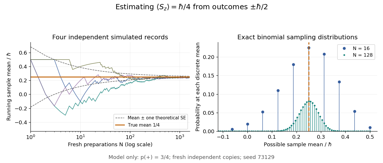
Repeatedly measuring one surviving system is a different protocol. Under the ideal Lüders rule, outcome leaves when . With no intervening change of observable or dynamics moving the state out of that eigenspace, the next projective measurement returns with certainty. Such a record is correlated and does not sample the original Born rule distribution independently. The quantum nondemolition measurement discussion describes this repeatability; fresh quantum state preparations supply the ensemble needed for the estimator above.
For spin one-half, choose the normalized spin eigenstates with . The spin one-half along an axis pure state in the plane isIts norm is one because the two eigenstates are orthogonal and . Applying the Born rule to a projective measurement givesConsequently the expectation value, second moment, and variance areAt , the outcome probabilities are and , the mean is , and the variance is . Every individual outcome remains . At , the mean is zero and the variance is maximal, . At either pole, one outcome has probability one and the variance vanishes.
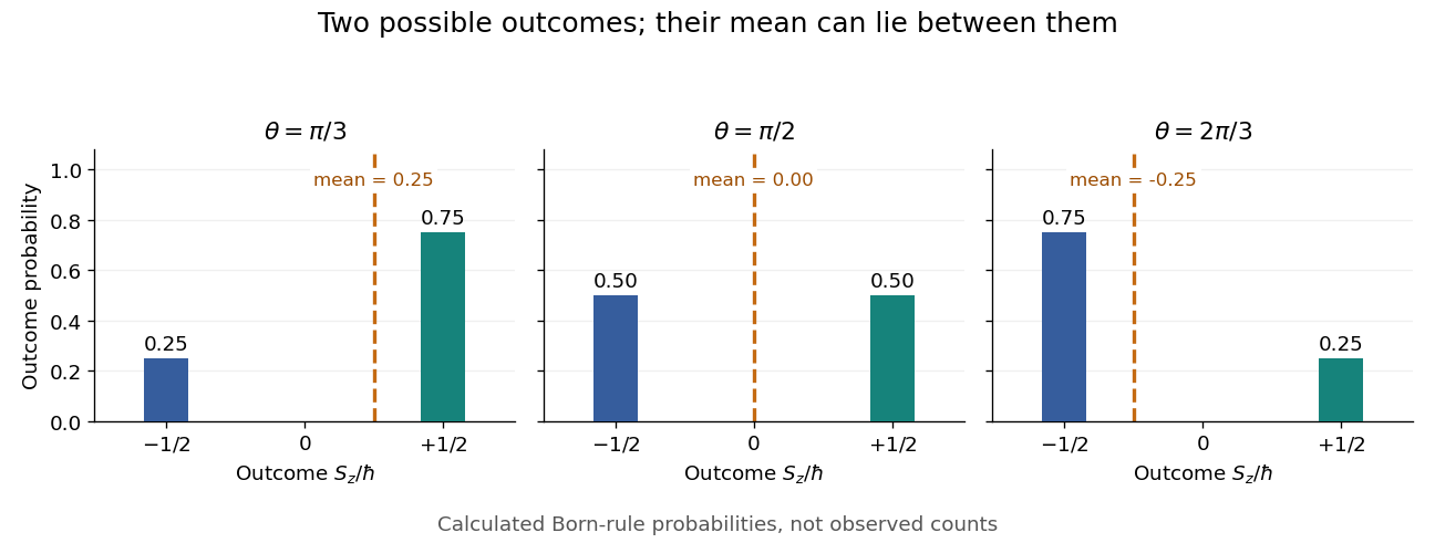
Spin expectation value between the two possible outcomes
. Original calculated Born rule distributions at three preparation angles. Bar heights are outcome probabilities; the dashed orange line marks the expectation value, whose horizontal position is usually not an allowed outcome. Spin values are expressed in units of the reduced Planck constant. No bars represent experimental observations. Source. Details.The diagonal mixed state has the same probabilities, expectation value, and variance as . It is nevertheless a different quantum state for : the displayed pure state has , while has . A single component's mean does not reveal all relative quantum phases or establish purity of a density operator.
For independent normal coordinates, an unobserved first coordinate has conditional law equal to its current marginal normal distribution, even when the second coordinate of that observation is known. Thus its E-step first moment is and second moment is . With three observed first coordinates and one missing value, the mean update is and the variance update is . The conditional variance term is essential: filling in only the conditional mean is not the expectation-maximization algorithm.
For a multinomial distribution with two unobserved cells merged into one observed count, the conditional allocation is a binomial distribution with probabilities proportional to the two cell probabilities. The expectation-maximization algorithm replaces the missing counts by their conditional expectations in the parameter-dependent part of the complete-data log-likelihood. The expectation of a log-factorial normalization generally differs from its value at the expected count, but this difference is independent of the candidate parameter and does not affect the maximization step.
For observations from each of two labeled exponential distributions, an E-step may produce positive completed time totals . Its expected complete-data log-likelihood is . This is strictly concave. On the closed ordering constraint , its maximum is when ; otherwise it lies at . To see the boundary case, first maximize along the equality line. At that maximum, moving into either feasible rate-separating direction has directional derivative , so concavity proves global optimality. For the open constraint , this boundary value is a supremum rather than an attained M-step.
// Target: probability-and-statistics.bigb
Choose six illustrative values , fixed mixture weights , known standard deviation , and initial means . These are constructed data for a Gaussian mixture distribution, not measurements. With the standard normal distribution probability density function, the fitted log-likelihood isAt the initial means, the component density ratio is . The first E-step therefore gives
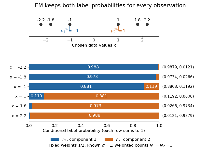
The paired values and have complementary mixture responsibilities, so exactly. The first M-step givesThe hyperbolic tangent expression follows by pairing the contributions at and . Assigning every negative value wholly to the first mixture component and every positive value wholly to the second would instead give means . Those hard assignments discard the overlap: the expectation-maximization algorithm is not the same update as K-means clustering.
The observed-data log-likelihood rises from initially to after one update and after two. Further updates approach means , with log-likelihood approximately . These values describe this initialization; EM likelihood monotonicity supplies no certificate of a global maximum.
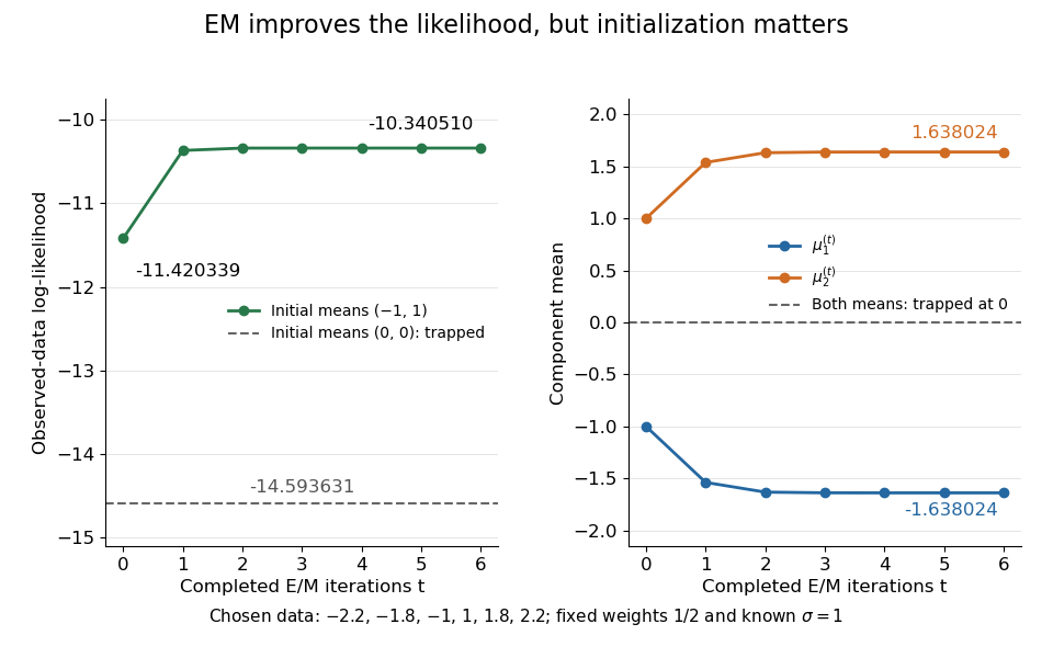
Likelihood ascent and mean updates for the chosen data, compared with an identical-means initialization
. Iteration zero is the initial fit; each subsequent point follows one E-step and one M-step. Starting at minus one and one increases the likelihood. Starting both means at zero leaves them at zero with a lower constant likelihood. All runs keep variance one and weights one half. Details.For stable numerical evaluation, put and . The log-sum-exp function givesSubtracting keeps at least one exponential equal to one, avoiding the all-zero sum that direct evaluation of tiny component densities can produce.
Maximize over the permitted statistical parameters, with the E-step conditional distribution held fixed.[ref]
Maximum Likelihood from Incomplete Data via the EM Algorithm by Arthur Pentland Dempster and others. Section 2, printed p. 6: general maximization step
A finite mixture model hasFor normal distributions with known common variance and fixed positive mixture weights, only the means are fitted. Dropping terms independent of these candidate means givesThe derivative in is , and its second derivative is . Thus a positive weighted count gives a unique maximizing weighted mean. This is a maximization of the surrogate ; the observed-data log-likelihood need not be concave. Recompute the mixture responsibilities after updating the means. The broader EM for Gaussian mixtures with a common variance also estimates mixture weights and the shared variance.Hold the old statistical parameters fixed when taking the conditional expectation, while keeping the candidate statistical parameters variable:For independent observations in a finite mixture model, is a hidden component label. Bayes' theorem gives its mixture responsibilities:These posterior probabilities are the conditional expectations of the mixture allocation indicators; they turn hidden counts into fractional counts.[ref]
Maximum Likelihood from Incomplete Data via the EM Algorithm by Arthur Pentland Dempster and others. Section 4.3, printed pp. 15-16, especially the paragraph following equation (4.3.3): conditional indicator probabilities and weighted counts
They condition on a current fixed fit, rather than averaging over a posterior distribution of the statistical parameters. Taking the conditional expectation of the complete-data log-likelihood is essential: substituting a single guessed label, or merely substituting the conditional mean into a nonlinear complete-data expression, generally gives a different algorithm.A starspot is a relatively cool, dark region on a star's surface associated with a magnetic field. Starspots change the light curve as the star rotates. A planet crossing a starspot blocks less light than it would from an unspotted region, producing a local upward anomaly during an exoplanet transit; unocculted starspots can instead deepen the normalized exoplanet transit depth. They can also distort spectral lines and imitate a Doppler spectroscopy signal.
The fractional decrease in observed radiative flux during an exoplanet transit, relative to the out-of-transit baseline. For a uniform star, a dark planet, full disc overlap, and no transit dilution, the exoplanet transit depth is . For a nonuniform star it depends on the blocked specific intensity as well as the radius ratio.
An existential formula is an existential block followed by a quantifier-free formula, with remaining free variables serving as parameters. Truth is preserved by structure embeddings. Reflection of truth for every such formula defines an existential embedding.
On , put independent rate- Poisson processes on unoriented nearest-neighbour edges, and exchange their endpoint occupations at each mark. Its generator on cylinder functions is . Equal occupations do not change the state, and a particle next to a vacancy jumps across at rate . The stirring representation of symmetric exclusion constructs it for arbitrary initial configurations. The simple occupation-product product self-duality of symmetric exclusion requires symmetry and is not the ordinary duality of an asymmetric process.
Copper(I) oxide, , is a copper oxide semiconductor in which copper has oxidation state . The name distinguishes it from copper(II) oxide, ; the chemical formula matters when identifying the material in an optical experiment.
Its importance here is the resolved Exciton Rydberg series observed in the exciton absorption experiment in copper(I) oxide. An optical absorption resonance can occur below the unbound electron–hole threshold because an electron and an electron hole bind as an exciton. Resolving many resonances approaching that threshold tests the internal bound-state model rather than directly imaging electron–hole orbits. Sample temperature, strain, illumination and line resolution affect how far the series can be followed; the linked experiment describes those controls.
Invariant sigma-algebra of an exchangeable sequence by  Codex 0 Created 2026-10-14 Updated 2026-11-05
On the coordinate product space of a sequence, the invariant sigma-algebra consists of measurable events unchanged by every finite permutation of coordinates. Its definition is pointwise and does not depend on the probability law. An exchangeable law makes each such permutation measure preserving. events in the tail sigma-algebra are invariant because any finite permutation fixes every sufficiently late coordinate. Conversely, exchangeable invariant events are tail events modulo null sets.
For an infinite sequence of real exchangeable random variables, conditional on its invariant sigma-algebra of an exchangeable sequence, the coordinates are independent and identically distributed. In particular, for Borel sets ,Here is the core proof. Let denote invariance under permutations of coordinates . Symmetrization as conditional expectation identifies the empirical average of each indicator with its conditional expectation on . The reverse martingale convergence theorem gives its limit conditional on . Multiplying the averages sums over all ordered coordinate tuples, including repetitions. Symmetrization of the product itself sums over the distinct tuples. The fraction of repeated tuples is at most , so these bounded averages have the same limit. This proves the displayed factorization. Permutation invariance also makes the individual conditional laws identical. A regular conditional distribution on the real line packages that common law as a random probability measure, giving the equivalent mixture-of-iid formulation.
For a module homomorphism over a commutative ring , is injective if and only if every is injective, with ranging over maximal ideals. In a localization of a module, maps to zero exactly when some denominator satisfies . If is injective this gives , so the original fraction is zero. In general it identifies with . A nonzero element of has a proper annihilator, contained in some maximal ideal; it remains nonzero in that localization. Thus vanishing of all localized kernels forces . No finiteness or Noetherian assumption is required.
For two independent continuous samples of positive sizes under a common-distribution null, each -subset of ranks is equally likely. The smallest rank sum is , attained only by . The only subset with rank sum one larger is . Hence the exact lower tail at that threshold is . This follows directly by observing that any other change increases the sum by at least two.
For a degree-zero rational function regular on an open subset of projective space, each derivative is a regular homogeneous rational function of degree . These derivatives define a derivation with values in , hence a map from the Kähler differential sheaf. The last map is . On , put and use frame . The derivative of has coordinate vector with at , at and zero elsewhere. Those vectors form a free basis of the kernel of , proving exactness directly in every characteristic.
Pinned article: Introduction to the OurBigBook Project
Welcome to the OurBigBook Project! Our goal is to create the perfect publishing platform for STEM subjects, and get university-level students to write the best free STEM tutorials ever.
Everyone is welcome to create an account and play with the site: ourbigbook.com/go/register. We belive that students themselves can write amazing tutorials, but teachers are welcome too. You can write about anything you want, it doesn't have to be STEM or even educational. Silly test content is very welcome and you won't be penalized in any way. Just keep it legal!
Intro to OurBigBook
. Source. We have two killer features:
- topics: topics group articles by different users with the same title, e.g. here is the topic for the "Fundamental Theorem of Calculus" ourbigbook.com/go/topic/fundamental-theorem-of-calculusArticles of different users are sorted by upvote within each article page. This feature is a bit like:
- a Wikipedia where each user can have their own version of each article
- a Q&A website like Stack Overflow, where multiple people can give their views on a given topic, and the best ones are sorted by upvote. Except you don't need to wait for someone to ask first, and any topic goes, no matter how narrow or broad
This feature makes it possible for readers to find better explanations of any topic created by other writers. And it allows writers to create an explanation in a place that readers might actually find it.
Figure 1. Screenshot of the "Derivative" topic page. View it live at: ourbigbook.com/go/topic/derivativeVideo 2. OurBigBook Web topics demo. Source. - local editing: you can store all your personal knowledge base content locally in a plaintext markup format that can be edited locally and published either:This way you can be sure that even if OurBigBook.com were to go down one day (which we have no plans to do as it is quite cheap to host!), your content will still be perfectly readable as a static site.
- to OurBigBook.com to get awesome multi-user features like topics and likes
- as HTML files to a static website, which you can host yourself for free on many external providers like GitHub Pages, and remain in full control

Figure 2. You can publish local OurBigBook lightweight markup files to either OurBigBook.com or as a static website.
Figure 3. Visual Studio Code extension installation.
Figure 5. . You can also edit articles on the Web editor without installing anything locally. Video 3. Edit locally and publish demo. Source. This shows editing OurBigBook Markup and publishing it using the Visual Studio Code extension. 
- Infinitely deep tables of contents:




All our software is open source and hosted at: github.com/ourbigbook/ourbigbook
Further documentation can be found at: docs.ourbigbook.com
Feel free to reach our to us for any help or suggestions: docs.ourbigbook.com/#contact