Topics (384k) Articles (398k) Users (410) Discussions (242) Comments (383) Files (13k) New article

Consider a neutral monoprotic acid dissolved in water, with no added salts or other acids. Assume dilute ideal thermodynamic activities, fixed temperature, water thermodynamic activity one, and negligible self-ionization of water. Write for its analytical concentration, with , and for its weak acid dissociation fraction. Conservation of acid units and electric charge givesHere is the conjugate base, and is conventional shorthand for hydrated hydrogen ions, represented by hydronium in this model. Substitution into the dimensionless acid dissociation constant givesSolving this quadratic equation and rejecting its negative root of a polynomial gives an exact result within the stated model:The second form avoids subtracting nearly equal numbers. Unlike the approximation , it retains depletion of neutral weak acid and always satisfies for positive . The broader weak acid mass and charge balances restore self-ionization of water when that omitted contribution matters.
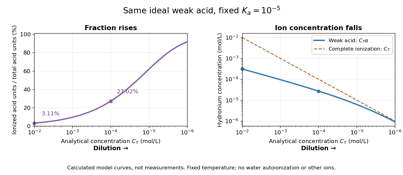
Dilution increases the ionized fraction while decreasing the absolute hydronium concentration in an ideal weak electrolyte model
. Original calculated curves for stipulated dimensionless acid dissociation constant at fixed temperature, not measurements of a named chemical acid. The shared horizontal analytical concentration axis decreases to the right. Separate panels show weak acid dissociation fraction and ; a dashed comparison shows a completely ionized monoprotic acid at the same . Both omit self-ionization of water, other ions and nonideal thermodynamic activities. Details.For an original worked example, stipulate without identifying a real substance. At , the weak acid dissociation fraction is approximately , or , and . A hundredfold dilution to raises the fraction to , or , but lowers to . A completely ionized strong acid at would have : less than the more concentrated weak acid in the first calculation, despite its greater converted fraction.
The directions of both changes follow without relying on the plot. Put . Rearranging the chemical equilibrium relation givesThus smaller forces smaller , which in turn makes larger. The derivative proves that total hydronium concentration and converted fraction move in opposite directions during dilution. In this model, adding solvent also makes additional acid units ionize at fixed total acid amount of substance, even though their ions are spread over more volume. That distinction explains why “more ionized” alone does not predict greater electrical conductivity.
Do not extend the no-background model to unlimited dilution: its prediction omits water's own ions. The weak acid mass and charge balances include that background. Added salts, other acids or bases, and nonideal activity coefficients also change the relation between analytical concentration, converted fraction and hydronium concentration.
Ion-channel inactivation is loss of availability for conduction, distinct from simply closing an otherwise activatable ion channel. Recovery depends on channel type and membrane potential; incomplete recovery of sodium-selective voltage-gated ion channels contributes to a neuronal refractory period.
The cover of the 2021 Chemical Demonstrations Booklet credits Tim Harrison and Magdalena Wajrak as its preparers.
For the normal sample sum with known variance, assume independent and identically distributed with fixed known variance . The joint probability density factors asThe Fisher-Neyman factorization theorem proves that the sum, and hence the sample mean, is a sufficient statistic for . Its remaining deviations have a joint Gaussian law independent of and are independent of . If both and are unknown, the sample mean alone loses information about variance; the pair is sufficient for the full statistical parameter.
A discrete counterexample shows why a sample mean is not automatically sufficient for arbitrary statistical models. Let be independent and identically distributed on withEach observation has mean one. The arrangements all give sample mean one, yetThis conditional probability is at and at . The conditional distribution therefore still depends on the unknown statistical parameter: this sample mean is not a sufficient statistic. The useful reduction depends on the family of full-data laws, even when its mean stays fixed.
A sufficient statistic allows the observed likelihood function to be stored through a shorter record, up to a parameter-independent factor. For the Bernoulli sample sum as a sufficient statistic, writeThe second likelihood function belongs to the observed count; the first belongs to the observed sequence. Their absolute values differ by the binomial coefficient, but their likelihood ratios between any two interior parameter values agree. A maximum-likelihood estimator can therefore use just .
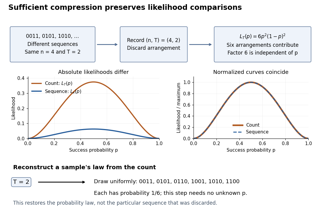
Sequence to count: sufficient compression preserves likelihood comparisons
. For , three example sequences share . Recording produces the count likelihood . Normalizing each curve by its maximum makes the two curves coincide. A reverse random draw from the six arrangements restores the full-data probability distribution, using no unknown . Details.This compression discards which arrangement actually occurred. To reproduce the original experiment's probability distribution, first draw from its binomial distribution and then draw uniformly from the arrangements with that sum. The second step is independent of , so it supplies no additional evidence about . It does not recover the particular discarded sequence. If the scientific question changes to time trends or statistical dependence between observations, the common- independent and identically distributed Bernoulli model may no longer apply, and the ordering can become informative.
Let be fixed and known, and let be independent and identically distributed Bernoulli random variables with common success probability . Their joint probability mass function, on the binary sample space , isThere are arrangements with successes, so has the binomial distribution. For and , its exact conditional full-data probability mass function isThis conditional distribution is uniform over arrangements, with no dependence on : the sum is a sufficient statistic. [ref]
Sufficiency (Stat 210a, Fall 2025) by Will Fithian. Sufficiency, Will Fithian, “Independent Bernoulli sequence”: conditional pmf
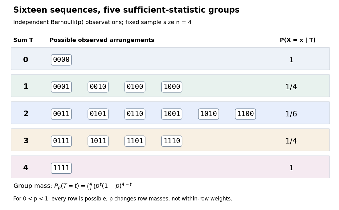
Four Bernoulli observations grouped by their sufficient sum
. All sixteen binary sequences are grouped by . Within each group the conditional distribution is uniform; changing changes the group's total probability, not the conditional weights within it. Details.For , the group sizes are and the within-group conditional probabilities are respectively . For example, leaves exactly , each with conditional probability . At , each such sequence has unconditional probability and the group has probability . At , these values are and ; at they return to and . The conditional weights stay in all three cases.
At the boundary , only has positive probability; at , only does. Dividing by on the other groups would divide by zero. Nevertheless, the same uniform-on-arrangements Markov kernel is a valid common version for the entire family : it gives the correct point mass on the one observed group at each boundary and assigns permissible versions on its unobserved groups. Define the joint probability mass function there by the original product of the one-trial Bernoulli probability mass functions, or use the limiting convention in the compact formula.
The sample mean is an unbiased estimator of and retains the sufficient statistic because is known. By contrast, is also an unbiased estimator of but, for , is not sufficient: the conditional success probability of the independent given is still . Thus unbiasedness does not imply sufficiency.
Sufficiency also does not imply completeness of a statistic. For , the full-data sufficient statistic admits the nonzero function with expectation zero for every . Nor does minimality imply completeness of a statistic: for and the restricted statistical model , is a minimal sufficient statistic since the likelihood ratio distinguishes its three values. Yet has expectation at both parameter values and is never zero. Changing the parameter family can change completeness of a statistic even while preserving sufficiency.
A spreadsheet cell reference identifies the spreadsheet cell read by a spreadsheet formula. In A1 notation,
B3 combines a column letter with a row number. For copying, the column and row can each be relative or absolute, independently: a $ immediately before a coordinate fixes that coordinate during the copy. The $ is an addressing marker, not a currency symbol. [ref]Switch between relative, absolute, and mixed references, Microsoft Support. Switch between relative, absolute, and mixed references: opening paragraphs and table of reference changes when copying two cells down and two cells right
Number columns as , , and so on. If a spreadsheet formula moves by columns and rows during copying, a referenced coordinate becomeswhere each is for a relative coordinate and for an absolute coordinate. This is a translation on the unfixed coordinates. For ordinary in-sheet references whose translated addresses exist, repeated copies compose by addition of their displacements: substitute the rule twice to obtain , and likewise for the row. Copying therefore preserves either a fixed coordinate or an offset from the formula's location.
Consider an original toy AB salt model with stipulated at fixed temperature and fixed activity coefficient product. This is a conditional concentration constant, not measured data for calcium carbonate or any identified material. A stock contains A cations and X anions; another contains Y cations and B anions. All four ions have unit electric charge magnitude. Only AB can form a solid; X and Y remain spectator ions. Assume full dissociation, no other chemical reactions, and a mixed volume equal to the sum of the initial volumes.
Mix two stocks, each of volume ,, each at molar concentration of its indicated salt. Before any precipitation, the mixed volume is , soMultiplying the two stock concentrations would overestimate the mixed ion product by a factor of four. The saturation threshold is .
If , mixing gives : no AB precipitate is favored. If , mixing gives . Suppose nucleation occurs and bulk AB solid remains at chemical equilibrium. Equal starting inventories and one-to-one stoichiometry require equal remaining concentrations, henceFor two portions in the second case, each reacting ion starts with ; the final chemical solution retains of each, and of AB enters the solid. The respective X and Y inventories stay at . Exactly half of each reacting inventory precipitates in this toy model.
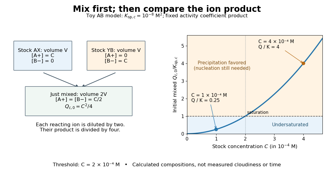
The chemical equilibrium calculation adds a phase constraint to the inventory balance. Write and . In the equilibrated bulk model,When , the last condition requires saturation; when , the inventory can leave an undersaturated chemical solution. Together these give . This excludes a persistent supersaturated solution by its explicit chemical equilibrium assumption; it does not model a nucleation delay.
Relative to the specified solid, favors dissolution if that solid is available; favors precipitation; equality marks saturation. These comparisons identify a driving direction favored by thermodynamics, not a reaction rate.[ref]
15.1 Precipitation and Dissolution. Chemistry 2e, §15.1, Predicting Precipitation: unsaturated, saturated and supersaturated cases
A proof outline comes from the reaction Gibbs free energy for dissolution:Here is the molar gas constant and the absolute temperature. If , the logarithm is positive, making the reverse transfer into solid favorable. At equality the bulk driving difference vanishes. Equality can also occur at the boundary where the last solid disappears, but it is not a universal constraint on every solid-free chemical solution.
Pinned article: Introduction to the OurBigBook Project
Welcome to the OurBigBook Project! Our goal is to create the perfect publishing platform for STEM subjects, and get university-level students to write the best free STEM tutorials ever.
Everyone is welcome to create an account and play with the site: ourbigbook.com/go/register. We belive that students themselves can write amazing tutorials, but teachers are welcome too. You can write about anything you want, it doesn't have to be STEM or even educational. Silly test content is very welcome and you won't be penalized in any way. Just keep it legal!
Intro to OurBigBook
. Source. We have two killer features:
- topics: topics group articles by different users with the same title, e.g. here is the topic for the "Fundamental Theorem of Calculus" ourbigbook.com/go/topic/fundamental-theorem-of-calculusArticles of different users are sorted by upvote within each article page. This feature is a bit like:
- a Wikipedia where each user can have their own version of each article
- a Q&A website like Stack Overflow, where multiple people can give their views on a given topic, and the best ones are sorted by upvote. Except you don't need to wait for someone to ask first, and any topic goes, no matter how narrow or broad
This feature makes it possible for readers to find better explanations of any topic created by other writers. And it allows writers to create an explanation in a place that readers might actually find it.
Figure 1. Screenshot of the "Derivative" topic page. View it live at: ourbigbook.com/go/topic/derivativeVideo 2. OurBigBook Web topics demo. Source. - local editing: you can store all your personal knowledge base content locally in a plaintext markup format that can be edited locally and published either:This way you can be sure that even if OurBigBook.com were to go down one day (which we have no plans to do as it is quite cheap to host!), your content will still be perfectly readable as a static site.
- to OurBigBook.com to get awesome multi-user features like topics and likes
- as HTML files to a static website, which you can host yourself for free on many external providers like GitHub Pages, and remain in full control

Figure 2. You can publish local OurBigBook lightweight markup files to either OurBigBook.com or as a static website.
Figure 3. Visual Studio Code extension installation.
Figure 5. . You can also edit articles on the Web editor without installing anything locally. Video 3. Edit locally and publish demo. Source. This shows editing OurBigBook Markup and publishing it using the Visual Studio Code extension. 
- Infinitely deep tables of contents:




All our software is open source and hosted at: github.com/ourbigbook/ourbigbook
Further documentation can be found at: docs.ourbigbook.com
Feel free to reach our to us for any help or suggestions: docs.ourbigbook.com/#contact