Topics (384k) Articles (398k) Users (410) Discussions (242) Comments (383) Files (13k) New article

A progenitor cell is a precursor with relatively restricted cell differentiation potential and, generally, more limited self-renewal than a stem cell. Usage depends on the lineage and assay; an expression marker alone does not establish renewal capacity.
A stem cell can produce both renewed stem cells and differentiated descendants. Its developmental range depends on the type and setting; self-renewal does not imply unrestricted cell fate.
A cell state describes current properties of a biological cell, including its gene expression, structure and activity. A snapshot of cell state does not alone establish its future cell fate.
Spontaneous emission is radiative decay of an excited matter quantum state by emission of a photon, without an applied resonant drive. In a simple Markov decay model the excited-level population obeys . During driven control, the expected emission count is governed by ; suppressing the lossy level's population is therefore the purpose of dark-state adiabatic transfer.
The statistical weight of an atomic level counts its degenerate quantum states. With no external field resolving magnetic substates, a specified total angular momentum gives states. An unresolved term can have a larger summed weight. These weights enter the Boltzmann distribution, Saha ionization equation and detailed-balance relations; term and resolved-level weights must not be interchanged.
An atomic oscillator strength is a dimensionless measure of an optical transition's absorption strength relative to a classical electron oscillator. It is related to its spontaneous radiative rate through the transition energy and the statistical weights of the two levels. The absorption convention fixes the lower state and upper state ; interchanging that convention can lose a weight factor.
A collisional-radiative model solves coupled atomic population equations using collisions, radiative transitions, ionization and recombination. For one fixed ion stage, a common stationary approximation is , supplemented by the total ion population. Electron-impact rates contribute and spontaneous downward transitions contribute . Additional radiation, proton collisions and adjacent-ion source terms are included when significant.
A metastable atomic level has no strong allowed radiative decay and therefore a comparatively long radiative lifetime. Weak multipole decays can still occur. At low density radiative decay can keep its population small; as density increases, collisional population and mixing compete with that decay. Metastable levels provide density-sensitive feeding of other spectral lines.
Fine structure splits atomic levels through relativistic corrections and interactions involving spin, such as spin-orbit coupling. Different total angular momenta can then have distinct energies. Even a small ground-term splitting can matter for density-sensitive metastable atomic levels, because weak radiative decay between the levels competes with collisional mixing.
Johannes Kepler inferred quantitative laws of planetary motion from astronomical observations. In Astronomia nova by Johannes Kepler, published in 1609, the problem of Mars's path led him to an ellipse with the Sun at one focus and an equal-area timing law.
The equal-area law states that the line from the Sun to the planet sweeps out equal areas in equal times. Together, a geometric orbit and a timing law specify where the planet moves and how its speed changes. Their later connection to a central force and an inverse-square law is explained in inferring an inverse-square force from Kepler laws; those dynamical deductions should be distinguished from Kepler's original empirical construction.[ref]
Astronomia nova by Johannes Kepler. Mars investigation and the first two planetary laws; digitized 1609 primary book

Portrait of Johannes Kepler
. Artist unknown; Photographische Gesellschaft Berlin reproduction, Smithsonian Libraries; file dates underlying portrait to 1620. Public domain (life+70 and U.S. pre-1931 publication tags). Source and usage information on the linked Wikimedia file page. Source.Edmond Halley connected separate historical appearances of a comet by comparing their calculated orbits. In his 1705 synopsis he argued that the appearances of 1531, 1607 and 1682 belonged to the same returning body.
The important step was a testable prediction: the comet should return, with its timing affected by gravitational perturbations from the planets. Its later return in 1758 supported the interpretation. The achievement applied orbital dynamics to historical observations rather than treating each bright apparition as an unrelated event.[ref]
A Synopsis of Cometary Astronomy by Edmond Halley. 1705 synopsis: comparison of historical orbital elements and predicted return; first-edition specimen account

Portrait of Edmond Halley
. Library of Congress, Prints and Photographs Division, Miscellaneous Items in High Demand, LCCN2002708778. Public domain (life+100/pre-1931 U.S. publication). Source and usage information on the linked Wikimedia file page. Source.Proper motion describes the change in a celestial object's direction on the sky due to its motion relative to the observer. Its angular velocity differs from the annual stellar parallax signal caused by the observer's orbit.
Thus proper motion is an angular velocity, rather than a speed in kilometres per second. It describes the relative transverse motion of source and observer in a specified reference frame. A star moving towards us can have little proper motion, while a nearer star can show larger proper motion than a faster but more distant one. In the example above, the observed coordinate actually decreases over the first half-year, although is positive: the annual stellar parallax excursion temporarily outweighs the steady drift. A short observed displacement alone therefore need not estimate proper motion well.
Real catalogues give two proper motion components. For right ascension and declination , the angular velocities in perpendicular directions on the local sky areThe cosine factor accounts for the shorter east-west arc associated with a given right ascension increment away from the celestial equator. ESA's Gaia DR3 fields
pmra and pmdec already contain these two components; pm is their total proper motion. Do not multiply pmra by another cosine. Components of and , for example, give total proper motion . [ref]https://gea.esac.esa.int/archive/documentation/GDR3/Gaia_archive/chap_datamodel/sec_dm_main_source_catalogue/ssec_dm_gaia_source.html. ESA Gaia DR3: Proper-motion columns and conventions
.For nearby stars in the ordinary nonrelativistic approximation, Euclidean distance converts total proper motion into transverse speed :The small-angle approximation gives transverse speed as Euclidean distance times angular velocity in radians per unit time. With arcseconds and parsecs, the parsec convention turns their product into astronomical units per year. One astronomical unit per Julian year of days is approximately . The coefficient is a unit conversion, rather than a property of a particular star.
Taking the model's as the total proper motion, with the other component zero, gives . At the same total proper motion, Euclidean distances of , and parsecs instead give transverse speeds of , and , respectively. Their stellar parallax values are , and . The same annual angular displacement can therefore describe quite different journeys through space.
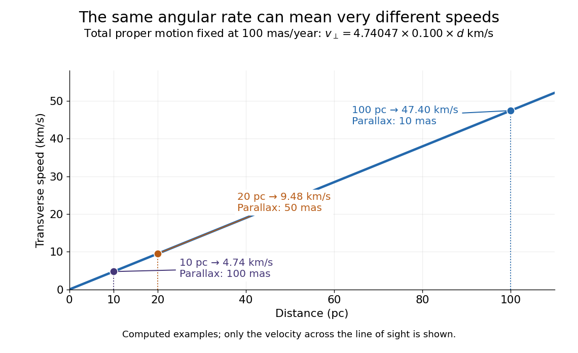
The transverse speed still omits the line-of-sight velocity, which can be measured through the Doppler effect in spectral lines. Combining these measurements permits a three-dimensional velocity estimate in a consistent reference frame. [ref].
Historically, Edmond Halley's 1718 paper compared contemporary and ancient stellar directions and argued that some supposedly fixed stars had moved. Its title, "Considerations on the change of the latitudes of some of the principal fixt stars", captures the conceptual surprise: long-separated measurements could reveal motion invisible in an ordinary night's watching. Modern astrometry retains that insight, using repeated precise measurements to turn the apparently static sky into a record of changing positions. [ref]
https://archive.org/details/paper-doi-10_1098_rstl_1717_0025. Halley: Original Royal Society paper, pages 736-738
. [ref]https://www.esa.int/Science_Exploration/Space_Science/Gaia/How_does_Gaia_study_the_Milky_Way. ESA: Halley's 1718 comparison
.Binary search finds a target in a sorted array by inspecting the middle of the remaining candidate range. If the middle entry is smaller than , every entry to its left is also too small; if larger, every entry to its right is too large. One comparison therefore rules out many entries. Equal entries are allowed; this version returns any matching index, without promising the first occurrence.
Use indices starting at zero and inclusive endpoints . Initially , , where is the array length. While , chooseThe brackets denote the floor function. Compare with : return on equality; set if ; otherwise set . If , report absence. The updates exclude the already inspected middle entry. This also handles an empty array, whose initial endpoints are . Sedgewick and Wayne specify a sorted array as input and return a matching index or for absence.[ref]
https://algs4.cs.princeton.edu/code/javadoc/edu/princeton/cs/algs4/BinarySearch.html. Sedgewick and Wayne: BinarySearch API
For , the first two steps agree. Next retains only index ; inspecting sets . Now , so the answer is "absent" after four comparisons.
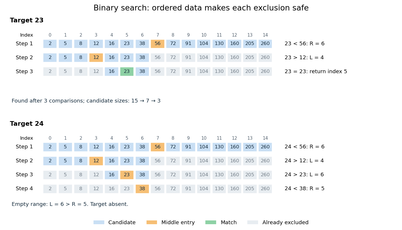
Binary search retains only candidates compatible with every comparison
. Blue cells are current candidates, orange marks the middle entry, and green marks a match. Both searches use the same fifteen-entry sorted array. Details.The loop invariant is: the array stays sorted, , and every index containing lies between and . It holds initially. The sorted array property justifies each exclusion. Returning on equality gives a match; an empty candidate range implies absence. Crucially, this loop invariant allows to be absent from the beginning.
For a nonempty range of size , an unsuccessful comparison leaves at most candidates. Thus sizes satisfy after unsuccessful comparisons. This proves termination and, for , at most middle-entry comparisons. The final singleton still needs inspection: requires one comparison, not zero. For , the bound is four. This is the halving argument behind logarithmic time complexity.[ref]
https://www.cs.princeton.edu/courses/archive/fall24/cos126/static/lectures/42Algorithms.pdf. Princeton COS 126: binary search analysis
A decision tree with binary tests has at most leaves. Distinguishing possible matching positions therefore requires . This lower bound counts binary tests, whereas the bound above counts three-way comparisons.
The merge algorithm combines two finite sorted sequences under the same total order, retaining every entry exactly once. Keep a position at the first unconsumed entry, or "head", of each input. While both heads exist, compare their keys, append the smaller head to the output, and advance only that head's position. On equality take the left head. Once either sequence is exhausted, append the other remainder without further key comparisons. Empty inputs therefore require no head comparisons. The MIT notes illustrate this two-head combination step.[ref]
Lecture 3: Insertion sort, merge sort. 6.006 Introduction to Algorithms, Fall 2011 by Massachusetts Institute of Technology, 6.006 course staff; MIT 6.006 (2011), lecture 3: merging sorted arrays
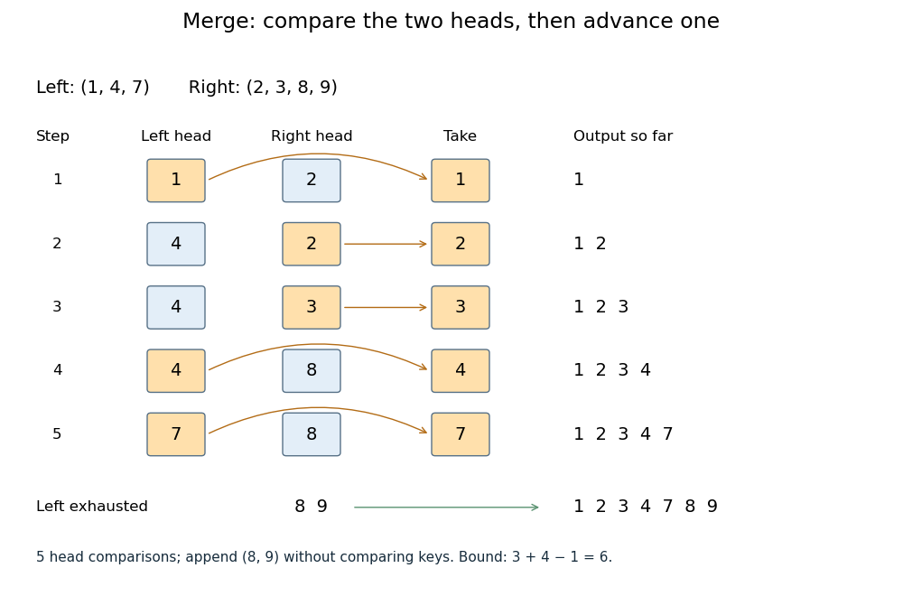
Five head comparisons in the merge algorithm
. Orange heads are chosen and arrows lead to the next output entry. The compared head pairs are (1,2), (4,2), (4,3), (4,8) and (7,8). The left sequence then runs out; append (8,9) without further key comparisons. Details.The head pairs , , , and select respectively. After the fifth comparison the left sequence is empty, so is appended. Seven entries are written, but only five head comparisons occur: tests for exhaustion and appending the remainder are separate operations. This distinction makes the example's count smaller than the bound .
For nonempty inputs of lengths , each head comparison consumes exactly one entry. After such removals at most one entry remains, so both heads cannot still exist. Hence the merge algorithm uses at most head comparisons. The bound can be attained: and require six head comparisons before the left sequence is exhausted. With constant-cost comparisons, access and copying, writing all entries gives time complexity in Big O notation. Writing a separate output array needs entry slots; the two positions require only constant additional storage.
The merge algorithm is useful whenever two already ordered collections must become one: it reads each input only forwards. This works with arrays and linked lists, without needing access to arbitrary middle positions. Choosing left on ties preserves each input's internal order and places equal left entries before equal right entries, which is the combination rule needed for stable sorting in merge sort.
The loop invariant behind algorithm correctness is that the emitted prefix is sorted, contains exactly the consumed entries, and every emitted key is at most every unconsumed key. Each sorted sequence has its smallest remaining key at its head, so the smaller of the two heads is safe to append. The invariant survives each removal; when one sequence ends, the other sorted remainder is safe to append in full. Each comparison removes an entry, so termination follows from the finite input lengths.
// Target: computer-science.bigb
A sorting algorithm rearranges a finite sequence into nondecreasing order under a chosen total order on its keys. Its output must contain every input entry exactly once, including repetitions: producing ordered values is insufficient if entries are lost. Merge sort is one such algorithm; stable sorting adds a requirement about equal keys.
Sorting creates reusable structure: equal sort keys become adjacent, and a sorted array supports binary search. However, an algorithm correctness check must establish both sortedness and sorting permutation preservation. Replacing every entry by the smallest key can produce ordered keys while destroying the original data. Stable sorting imposes a third condition when equal sort keys occur: retain their arrival order.
For example, take complete sorting records , with the first component as the sort key and the letter as associated data. A correct output is . The sort keys are ordered, every complete sorting record remains, and the equal-key pairs keep before and before . The output satisfies sortedness and sorting permutation preservation, but fails stable sorting. The output has the right multiset of sort keys but loses and duplicates ; it fails sorting permutation preservation of complete sorting records.
To express stable sorting precisely, label every input occurrence by its original position, even when two complete sorting records have identical contents. Let be the output position of the occurrence originally at position . Besides sortedness and sorting permutation preservation, requireHere is the sort key function. Sorting by the pair under lexicographic order gives the same order as stable sorting by : the original position breaks ties without discarding associated data. For a two-field ordering, first apply stable sorting by the secondary sort key, then apply stable sorting by the primary sort key. The second pass retains the secondary order within each group of equal primary sort keys. For instance, first becomes by letter, then by number.
A divide-and-conquer algorithm divides a problem into smaller instances, solves them using recursion, and combines their answers. In merge sort, the division makes two contiguous halves, and the merge algorithm combines the resulting sorted arrays. The important design step is finding a combination rule cheaper than solving the whole problem afresh.
Halving the input is only one part of the design. The number of recursive calls and the work outside those calls determine whether the smaller instances actually save time. Divide-and-conquer combination cost keeps these quantities separate; the divide-and-conquer product ledger shows how an algebraic identity changes the number of required calls in Karatsuba multiplication.
For algorithm correctness, specify the meaning of each returned answer, prove the base cases, and show that combining correct smaller answers gives the required output. Induction then proves correctness, provided every recursive call progresses towards a base case. The combination rule must reconstruct everything the caller needs: two sorted halves alone are not a sorted array, and four digit blocks alone are not their integer product.
Recursion solves a problem by invoking the same procedure on smaller instances, with base cases answered directly. For merge sort, an empty or one-entry array is already sorted, and every larger array is split into two shorter parts. The decreasing lengths justify termination; a self-call without a progress rule would not suffice.
A recursive procedure refers to itself, directly or through another procedure. A recursive call starts another invocation, with its own arguments and local variables; the caller can wait for its returned output. A base case supplies an answer without further recursive calls. To establish algorithm termination, also show that every recursive call progresses in a well-founded relation. “Smaller” means smaller in that chosen relation: argument values need not all decrease, and the arguments need not even be numbers.
Recursion is especially expressive when a data structure already decomposes into smaller structures. A binary tree has two child subtrees, so structural recursion can follow its shape. A short rule for each case can describe an entire traversal or computation. The distinction between a recursive procedure and the recursive process it generates helps connect that compact description to its resource use.[ref]
Structure and Interpretation of Computer Programs by Harold Abelson and others. Structure and Interpretation of Computer Programs, second edition, §1.2.1: procedure versus process; §1.2.2: closing discussion before Counting change, hierarchical data and straightforward definitions
Memoization retains a completed function result under a memoization key and returns that result when an equivalent request recurs. For a terminating pure function, repeated evaluation can therefore become lookup rather than repeated work. The benefit is especially striking with recursion and overlapping subproblems: a large tree of calls can refer to a small directed acyclic graph of distinct answers. The memoization cache contract determines whether reuse is correct; the memoization cache lifetime determines whether an answer is still present when wanted.
Memoization records computed answers, whereas a memory cache retains data from computer memory. A CPU cache hit does not by itself prevent a program from evaluating the same function again. Spreadsheet dependency evaluation adds an explicit mechanism for invalidating affected cached cell values after inputs change; a general memoization table does not discover such changes automatically.
A documented early motivation was to let programs improve their efficiency during execution through rote learning: the abstract of a 1968 paper explicitly proposes such a programming language facility.[ref]
“Memo” Functions and Machine Learning by Donald Michie. Donald Michie, “Memo” Functions and Machine Learning, Nature 218, pp. 19–22 (1968), abstract: programming-language rote learning motivated by efficiency during execution
Depth-first search is a graph search that follows a branch as far as it can before returning to try the next unexplored branch. Starting at a vertex of an undirected graph on a finite set of vertices, mark as discovered. Scan its graph neighbours in a fixed order: for each undiscovered vertex, record the current vertex as its parent in a rooted tree in the discovery tree, mark the new vertex, and explore it immediately using recursion. Return when its adjacency list is exhausted. Discovery marks persist after return, preventing a graph cycle from causing repeated exploration. This branch-and-return rule is the maze exploration described in MIT's notes. [ref]
Use the same unweighted undirected graph as breadth-first search, with vertex set and edgeswhere denotes the unordered pair . Visit graph neighbours in lexicographic order of their one-letter labels, starting at . The discovery order, computed by the diagram's generator, isThe discovery edges in order are . They form a rooted tree spanning the reached vertices, with root of a tree . The other edges, and , remain in the original graph but never discover a new vertex. In particular, the graph cycle causes no repeated discovery.
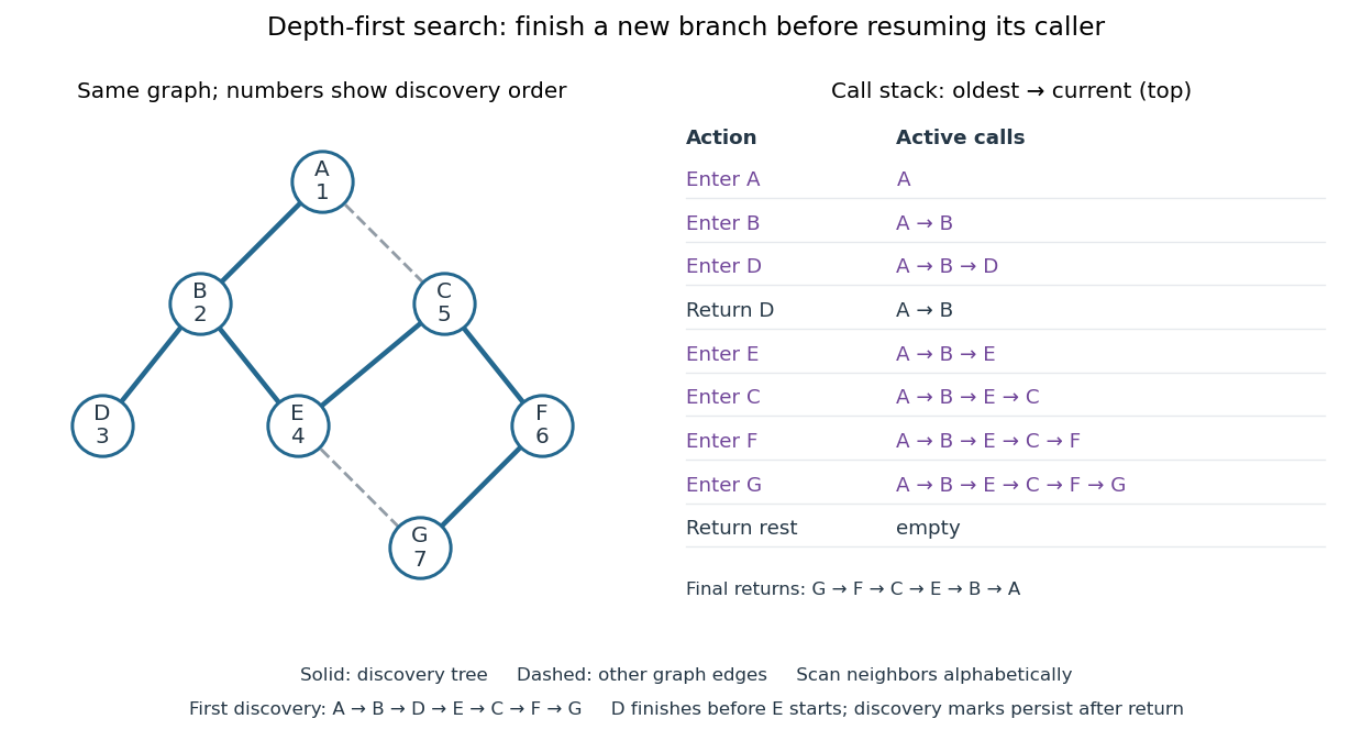
At there is no undiscovered graph neighbour, so its call returns to . The next call enters , then , then , then . Immediately after discovering , the call stack is , with on top; is still discovered but its call has finished. The maximum call stack depth is six, although seven vertices are discovered. Following the recorded parent in a rooted tree backwards at each step reconstructs a graph path; here the route from to is , using five edges. Breadth-first search instead finds , using three edges. Depth-first search establishes reachability but does not guarantee the fewest edges.
An explicit LIFO stack can replace recursion, but its entries and discovery rule must be specified. To reproduce this exact traversal, store one frame per active vertex, retaining the next position in its adjacency list. Advance the top frame by one graph neighbour; if that vertex is undiscovered, mark it and push its frame immediately; pop an exhausted frame. Pushing all undiscovered graph neighbours at once and marking them on push is a different iterative variant. Even pushing them in reverse lexicographic order does not generally reproduce the parent in a rooted tree relationships above: would already be marked while processing , so could not discover .
With an adjacency list representation, constant-cost discovery checks and frame operations, and the graph neighbours already ordered, depth-first search has time complexity in Big O notation. Each reached vertex is entered once and each incident edge is examined at most twice in an undirected graph; initializing all discovery marks costs . The call stack has depth at most , since no active vertex repeats. Discovery marks and the recorded parent in a rooted tree for each nonroot vertex also need auxiliary space complexity, excluding storage for the graph. Sorting adjacency lists to obtain a chosen order is additional work. [ref]
https://raw.githubusercontent.com/kevin-wayne/algs4/master/src/main/java/edu/princeton/cs/algs4/DepthFirstPaths.java. Sedgewick and Wayne, Algorithms: DepthFirstPaths discovery marks and resource bounds
One start explores only its connected component of a graph. To cover a disconnected graph, start again at every still-undiscovered vertex while keeping all discovery marks; the discovery trees form a forest. Depth-first search is useful for reachability, constructing a spanning tree of a connected graph, and organizing the return steps needed by a depth-first traversal of a tree. For detecting a graph cycle in a simple graph that is an undirected graph, an edge to an already discovered vertex other than the current parent in a rooted tree closes a graph cycle; the immediate return edge to that parent in a rooted tree is not itself a graph cycle.
// Target: computer-science.bigb
Pinned article: Introduction to the OurBigBook Project
Welcome to the OurBigBook Project! Our goal is to create the perfect publishing platform for STEM subjects, and get university-level students to write the best free STEM tutorials ever.
Everyone is welcome to create an account and play with the site: ourbigbook.com/go/register. We belive that students themselves can write amazing tutorials, but teachers are welcome too. You can write about anything you want, it doesn't have to be STEM or even educational. Silly test content is very welcome and you won't be penalized in any way. Just keep it legal!
Intro to OurBigBook
. Source. We have two killer features:
- topics: topics group articles by different users with the same title, e.g. here is the topic for the "Fundamental Theorem of Calculus" ourbigbook.com/go/topic/fundamental-theorem-of-calculusArticles of different users are sorted by upvote within each article page. This feature is a bit like:
- a Wikipedia where each user can have their own version of each article
- a Q&A website like Stack Overflow, where multiple people can give their views on a given topic, and the best ones are sorted by upvote. Except you don't need to wait for someone to ask first, and any topic goes, no matter how narrow or broad
This feature makes it possible for readers to find better explanations of any topic created by other writers. And it allows writers to create an explanation in a place that readers might actually find it.
Figure 1. Screenshot of the "Derivative" topic page. View it live at: ourbigbook.com/go/topic/derivativeVideo 2. OurBigBook Web topics demo. Source. - local editing: you can store all your personal knowledge base content locally in a plaintext markup format that can be edited locally and published either:This way you can be sure that even if OurBigBook.com were to go down one day (which we have no plans to do as it is quite cheap to host!), your content will still be perfectly readable as a static site.
- to OurBigBook.com to get awesome multi-user features like topics and likes
- as HTML files to a static website, which you can host yourself for free on many external providers like GitHub Pages, and remain in full control

Figure 2. You can publish local OurBigBook lightweight markup files to either OurBigBook.com or as a static website.
Figure 3. Visual Studio Code extension installation.
Figure 5. . You can also edit articles on the Web editor without installing anything locally. Video 3. Edit locally and publish demo. Source. This shows editing OurBigBook Markup and publishing it using the Visual Studio Code extension. 
- Infinitely deep tables of contents:




All our software is open source and hosted at: github.com/ourbigbook/ourbigbook
Further documentation can be found at: docs.ourbigbook.com
Feel free to reach our to us for any help or suggestions: docs.ourbigbook.com/#contact