The Linial-Mansour-Nisan theorem says that small constant-depth Boolean circuits have little high-degree weight in their Fourier expansion. Consider unbounded-fan-in AND gates and OR gates with negated inputs allowed. For fixed depth $d$, size $s$, and $0<\epsilon <1$, there is a cutoffsuch thatHere $f:\{0,1{\}}^n\to \{-1,1\}$, ${\chi }_S(x)=(-1{)}^{{\sum }_{i\in S}{x}_i}$ and $\hat{f}(S)=\mathbb{E}[f(x){\chi }_S(x)]$ under the uniform distribution on a finite set. The implicit constant is independent of $n,s,\epsilon$ for the fixed circuit model.^[ref]

Truncate the Fourier expansion to $p(x)={\sum }_{|S|\le t}\hat{f}(S){\chi }_S(x)$. Parseval's identity gives $\mathbb{E}[(f-p{)}^2]\le \epsilon$, so the Boolean function has a low-degree real polynomial approximation in mean square. This is an average-error statement for uniform inputs, not a pointwise approximation guarantee.

The full parity Boolean function is one character ${\chi }_{[n]}$, with all its weight at degree $n$. For fixed $d$ and polynomial $s$, the cutoff above is eventually smaller than $n$, contradicting the claimed small tail. Thus parity is outside polynomial-size constant-depth AC0 circuits. Concentration also makes low-degree coefficient estimation useful in computational learning theory.^[ref]

A programming language specifies how programs are written and what their execution means. Its type system describes which operations may be combined; an abstract syntax tree records the structure on which these rules act. The examples under type system use a small teaching language with integers, Boolean values and function types.

// Target: computer-science.bigb

A data structure organizes stored information together with operations for accessing and changing it. Choosing a data structure means choosing which questions should be cheap to answer: an array supports access by numbered position, a hash table supports lookup by key, and a priority queue supports selecting an item by priority. The operations and their time complexity matter as much as the stored values.

Suppose three requests arrive as $(5,\mathrm{Ada}),(2,\mathrm{Bo}),(4,\mathrm{Cy})$, where the number is a priority and smaller numbers are more urgent. A FIFO queue removes Ada first because she arrived first. A minimum-oriented priority queue removes Bo first because $2$ is the least priority. An array can store the same three records in arrival order, but finding the least priority by scanning this representation takes three key inspections. A binary heap organizes these records so the least priority is immediately available. The information is the same; the representation changes the work needed to use it.

This is a useful design principle: preserve just enough organization for the operations the application needs. Maintaining a sorted array gives the whole order, but moving entries to insert a new key can be expensive. A binary heap keeps a weaker heap order that supports fast repeated selection without maintaining a sorted array. A good data structure makes an algorithm's next step easy.

An operating system manages the resources that let programs run and cooperate. Operating-system processes organize running work, virtual memory supplies protected address spaces, and a file system supplies named files that can outlive the operating-system process that created them. The operating-system kernel enforces the core mechanisms; system calls let programs request its services. Separating these responsibilities makes it possible to share a file while keeping the participating operating-system processes' address spaces isolated. ^[ref]

A concrete example makes the separation useful: two operating-system processes can each use file descriptor 3, yet refer to different files; two different names can instead refer to the same file through hard links. Neither a name nor a small integer identifies an object without its context. Virtual memory has a related distinction: the same virtual address in different address spaces can designate different physical addresses.

Unix provides an influential example of this design. In their July 1974 paper, Dennis M. Ritchie and Ken Thompson date its earliest version to approximately 1969–70 and describe operating-system processes, a hierarchical file system, and inodes separating directory entries from file metadata. This is a documented historical example, rather than a claim that every operating system uses Unix conventions. ^[ref]

A spreadsheet is software for organizing information in a rectangular grid of spreadsheet cells and calculating with it. Rows are numbered and columns are lettered: B3 is the spreadsheet cell at column B, row 3. A spreadsheet cell can hold a label, a numerical input, or a spreadsheet formula whose value supplies an output. This brings a mathematical model close to its data: quantities, assumptions and results can be read side by side. The address convention is described in LibreOffice's official help. ^[ref]

The useful idea is to write a relationship once and reuse it across similar rows. Relative spreadsheet references follow each row's data; absolute spreadsheet references retain a shared assumption; mixed spreadsheet references let one coordinate vary while the other stays fixed. Spreadsheet dependency evaluation then computes the resulting spreadsheet formulas. A rectangular layout organizes the model for its reader, while the spreadsheet dependency graph organizes its calculation.

Spatial locality is the tendency to access nearby locations in computer memory within a short interval. A sequential scan of a contiguous array has spatial locality even when each element is read only once. A memory cache can exploit spatial locality by fetching a whole cache line on a cache miss: later reads of neighbouring elements become cache hits. Proximity is in the address layout, so visually adjacent entries in a table need not be adjacent bytes.

Consider a $4\times 4$ array of 32-bit integers, each occupying four eight-bit bytes, stored contiguously in row-major order. Use toy physical addresses starting at zero, aligned to a 16-byte cache line boundary. For row $i$ and column $j$, with $0\le i,j<4$, the address and cache block number areHere $\lfloor \cdot \rfloor$ is the floor function. Each row occupies exactly one cache line: row zero begins at addresses $0,4,8,12$, row one at $16,20,24,28$, and so on. Row-major order describes this storage layout; traversal can follow rows or columns without moving the elements.

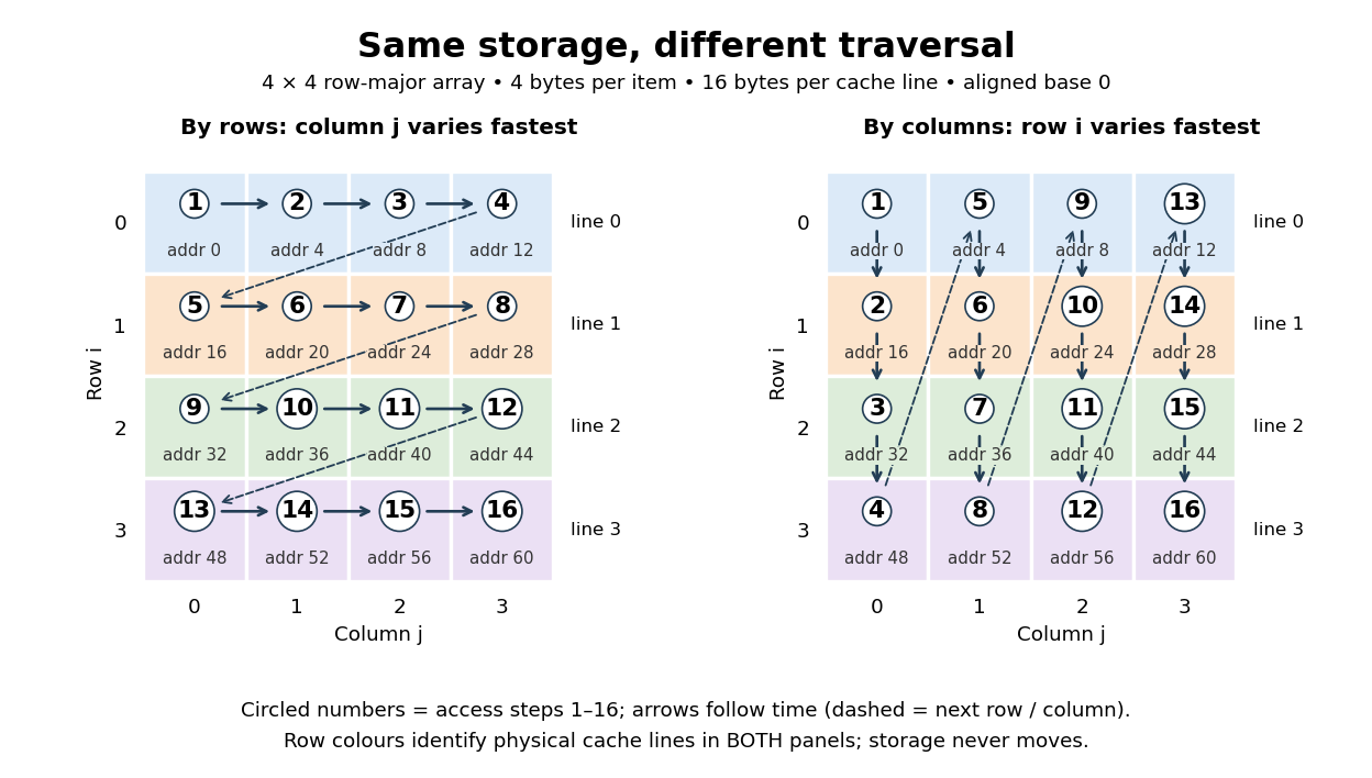
Read all sixteen elements and compute their integer sum, keeping the accumulator outside the modelled memory cache. Only the sixteen array reads count as memory references. The toy fully associative cache starts empty, holds exactly one 16-byte cache line, fetches the requested cache block on every cache miss, and uses LRU replacement. No cache block is fetched ahead of a request, and no writeback costs are counted because the modelled accesses are reads.

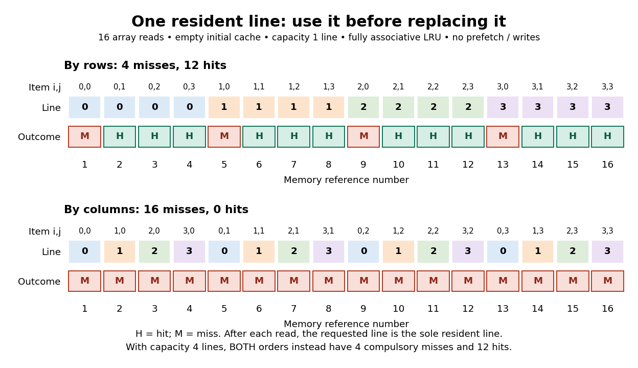
Every element is read once in both traversals. The row traversal exploits spatial locality between distinct elements and temporal locality of their shared cache block. The column traversal returns to each cache block after three other distinct cache blocks, too late for the one-line memory cache. Increase the fully associative cache to four cache lines and both traversals give four compulsory misses and twelve cache hits: no loaded cache block needs eviction. The difference therefore depends on capacity as well as access order and layout.

This makes spatial locality useful and beautiful: the same logical operation on the same elements can use a fetched cache line much more fully simply by changing traversal order. The toy counts do not predict a universal speed ratio on real hardware. Actual cache line sizes, capacities, placement rules, fetching ahead of requests and overlapping work affect runtime; measure a concrete implementation with statistical program profiling. Ulrich Drepper's November 2007 authored paper explains cache line transfers and gives array and matrix access examples connecting layout, temporal locality and spatial locality. Its hardware measurements are historical examples, rather than specifications for every present-day CPU. ^[ref]

// Destination: computer-science.bigb

Temporal locality is the tendency for the same item to be accessed again soon after an earlier access. For computer memory, the item might be an array element, a cache line or a memory page; always specify the unit. Temporal locality concerns reuse over time, whereas spatial locality concerns accesses to nearby addresses. Both are properties of a workload, rather than guarantees about its next memory reference. ^[ref]

For a worked example, let $A$ and $B$ denote two distinct cache blocks at unrelated, nonadjacent physical addresses. An initially empty fully associative cache holding two cache lines, with LRU replacement, receives the sequence $A,B,A$. The first $A$ causes a cache miss and leaves $A$ resident; $B$ causes another cache miss and leaves both $A$ and $B$ resident; the last $A$ is a cache hit. LRU replacement now regards $B$ as older than $A$. The benefit comes from temporal locality of $A$, irrespective of how far apart the cache blocks lie. With capacity one, the same sequence gives three cache misses: reuse helps only if the item survives until it is needed.

The appealing idea is that a small memory cache can serve a large computation when its currently useful data stay small. Repeatedly reading a counter or executing the same instructions can exploit temporal locality. LRU replacement and recency-based approximations try to retain recently used items. A working set records recent demand; if the active working set cannot fit in resident memory pages, memory thrashing can defeat this benefit. At cache line granularity, even accesses to different array elements can reuse the same cache block, as the spatial locality example shows.

Peter J. Denning's May 1968 paper connected recent memory page use to near-future demand through the working set. Section 3 explicitly discusses the clustering of references to the same memory page in time. This is a documented early treatment of the reasoning behind temporal locality, rather than a claim about who first coined the term. ^[ref]

Transfers of data between a computer and its devices or external environment. An operating-system process can need to wait for an input-output operation to complete, leaving the CPU available for other runnable work. Polled input-output, interrupt-driven input-output and DMA describe different aspects of arranging and observing such transfers.

// Destination: computer-science.bigb

The processor executing a program's instructions. In polled input-output the CPU explicitly checks status; in interrupt-driven input-output it enters an interrupt handler; in DMA it delegates payload movement while retaining setup and completion work.

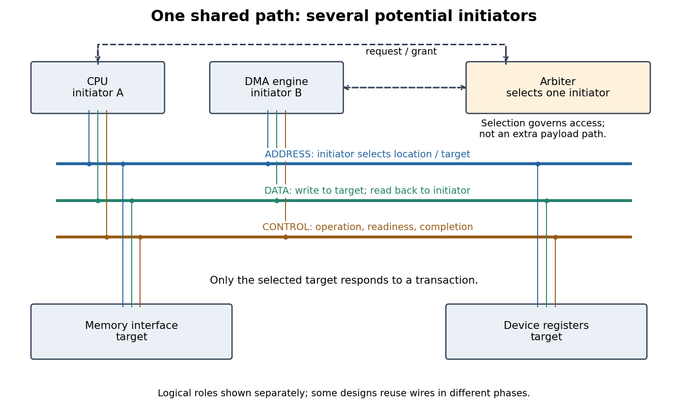
A computer bus connects components through agreed communication paths and transfer rules. On a shared computer bus, a CPU and a DMA engine can both want the same path to computer memory: attaching another initiator does not create another independent path. Bus arbitration chooses who may start; bus ownership states who may use each resource; bus throughput measures the useful data delivered. This makes sharing a performance question as well as a correctness question.

A processor register identifying the current or next instruction according to the architecture. A timer interrupt can record the saved instruction address of a running process, permitting statistical program profiling without source code.

// Destination: computer-science.bigb

A cellular automaton assigns one of finitely many states to each cell of a regular grid and updates cells in discrete generations using a fixed local rule. In the synchronous convention, each new state depends only on old states in a finite neighborhood. Conway's Game of Life supplies a concrete example with two states and eight neighbors; its global update is a function on complete configurations, with deterministic evolution.^[ref]

// Destination: foundations-of-mathematics.bigb

Conway's Game of Life is a cellular automaton in which a simple local rule produces patterns that remain still, pulse, or travel across a square grid. Choose the starting pattern; after that there are no player decisions. The Life blinker and Life glider below make the surprise concrete: the rule mentions only births and survival, yet repeated applications create a clock and a moving shape.

The standard board is infinite, with cells at ordered pairs $(x,y)\in {\mathbb{Z}}^2$ of integers. At generation $t\in \{0,1,2,\dots \}$ let $a_t(x,y)$ be $1$ for a live cell and $0$ for a dead cell. Count all eight cells sharing an edge or a corner, excluding the center itself:The local Boolean function defining the next generation isThis is the rule B3/S23: a dead cell is born with exactly three live neighbors; a live cell survives with exactly two or three. A live cell with zero or one, or with four through eight, dies. A dead cell with two stays dead. All counts and center states come from generation $t$: this is a synchronous update, even if an algorithm computes its cells one at a time.^[ref]

In particular, the two births in the Life blinker do not help any other cell survive until the following generation. Writing each answer over its old value and then reading that new value for another count changes the rule. The simplest correct algorithm reads one array and writes the next generation into a second array; swap their roles after the entire step. The one-row in-place Life update achieves the same rule with less auxiliary storage by preserving the old values that later counts still need.

A finite implementation must specify its boundary convention. Holding all cells outside the rectangle permanently dead can destroy a Life glider when it reaches the edge. Wrapping neighbor coordinates from one edge to the opposite edge allows interaction with patterns on the other side. Neither convention is the infinite board. The figures display finite windows into an infinite board initially dead everywhere except the stated live cells; the windows do not impose walls.

Conway's Game of Life illustrates emergence in a precise, modest sense: the Life glider's motion is a collective pattern derived from local birth and death, without a motion command. It has deterministic evolution; visually surprising behavior introduces no random choices. Nor do the words "alive" and "dead" make it an experimentally validated model of biology. The beauty is that the same rule yields a stable four-cell square, the Life blinker, and the Life glider: three qualitatively different behaviors from a handful of cells.

For the stable square, take the live set $\{(0,0),(1,0),(0,1),(1,1)\}$. Each live cell has three live neighbors, and every dead cell has at most two. The next generation is identical: this configuration is a fixed point of the global update function. In contrast, the Life blinker returns after two generations, and the Life glider returns only after allowing a translation.

The patterns are useful as small, exact checks of an algorithm: the square checks survival without births, the Life blinker checks births and deaths in one simultaneous step, and the Life glider checks several steps and diagonal neighbors. More elaborate constructions can encode data and assemble Boolean circuits; Johnston and Greene develop constructions that simulate arbitrary computation in their chapter 9. This is a statement about suitably designed patterns with enough space and time, not a claim that every starting pattern computes something useful or that a fixed finite board has unlimited computer memory.^[ref]

Martin Gardner introduced Conway's Game of Life to his Scientific American readers in October 1970, reporting that Conway selected the rules after experimentation with patterns. The aim was sustained, varied behavior rather than immediate extinction or trivially demonstrable unlimited growth. These were mathematical explorations of chosen rules.^[ref]

Gardner's hands-on procedure is still a useful experiment: place black counters for the current live cells; mark doomed counters by stacking another black counter; mark births with white counters; finish checking before removing the doomed stacks and turning white counters black. Count only the original black occupants. Repeat with three adjacent counters to obtain the Life blinker, then with the five coordinates of the Life glider. Recording each generation tests whether the procedure implements the rule; it does not measure a natural population.^[ref]

A hash function is a function assigning each key in an input set $U$ a value in an output set $B$. Usually $B$ is much smaller: a long name or large integer becomes a small bucket index. Equal keys must receive equal values from the same hash function; different keys may also receive equal values. Such a hash collision means "look in the same place", and does not establish key equality. If $|U|>|B|$, the pigeonhole principle makes some collisions unavoidable.

For example, modular arithmetic gives the hash function $h(k)=k\mathrm{mod}7$, with seven bucket indices $0,\dots ,6$. Store the seven keys $0,2,3,10,11,17,24$: their values are respectively $0,2,3,3,4,3,3$. In particular, $h(3)=h(10)=3$ although $3\ne 10$. A hash table is a data structure that uses these indices to locate records. With separate chaining, each bucket holds a linked list of records, so bucket $3$ retains all four keys $3,10,17,24$. Inserting $10$ must not overwrite $3$ merely because their hash function values agree.

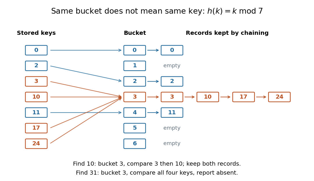
Searching for $10$ computes bucket $3$, then compares the actual keys until it reaches $10$. Searching for absent key $31$ reaches that same bucket and must reject every stored key. This data structure trades a search through all records for a search through one short chain, provided the hash function distributes keys adequately. A fixed hash function can perform poorly on patterned keys: $3,10,17,24$ already demonstrate the problem. A universal hash family introduces controlled randomness to limit the expected value of this extra work. Neither indexing nor a small collision probability inherently supplies encryption or message authentication; a cryptographic hash function has additional requirements such as collision resistance.

Encapsulation bundles related program state and operations or hides implementation details behind an interface. Encapsulation in object-oriented programming realizes this through objects and their permitted operations; encapsulation also applies to modules outside object-oriented programs.

The useful boundary is a promise: clients request operations through an API, and the implementation maintains a representation invariant. Instead of proving that every client updates several storage fields consistently, prove that the permitted operations preserve the representation invariant. Information hiding also leaves room to replace the data structure while keeping the client-facing behavior, a property called representation independence.

Bundling state and operations alone does not establish that promise. Representation exposure can let clients bypass the API. A private annotation alone is not a security guarantee: it does not establish correctness of operations, isolation from hostile code or safe handling of shared mutable storage. The examples below concern sequential calls with no concurrent access and no client access to internal storage; they do not claim protection against arbitrary memory modification.

A software module groups responsibilities behind an application programming interface. Its boundary can be maintained by procedures and hidden storage; it need not be a class in object-oriented programming. Information hiding guides which implementation decisions belong inside that boundary.

Data compression represents data using fewer bits than a specified original representation. The saving can reduce storage in a file system and reduce the number of bits sent through a communication channel. At a fixed transmission rate, fewer bits arrive sooner; this makes better use of a fixed transmission budget. Both the encoded data and the instructions needed to interpret them contribute to the size of a stored file.

There are two different promises. Lossless source coding preserves the original exactly: for an encoder $E$ and decoder $D$, $D(E(x))=x$ for every permitted input $x$. Thus $E$ must be an injective function. Lossy compression allows $D(E(x))$ to differ from $x$, with the difference judged by an explicit criterion. A program or numerical record may require exact recovery; a preview image may tolerate altered pixels in return for fewer bits.

The appeal of lossless source coding is that repetition can be described rather than copied. Run-length encoding says "repeat this value twelve times"; a prefix code can give more frequent symbols shorter descriptions. These are distinct ways to exploit structure, and neither promises savings for every input. Image compression supplies especially visible examples of both lossless source coding and lossy compression.

Claude E. Shannon's 1948 paper made the role of probability distributions precise. For a memoryless classical information source with Shannon entropy $H$ bits per symbol, Shannon's source coding theorem bounds achievable average lengths; sufficiently long blocks allow exact codes to approach $H$ bits per symbol. This is a statement about a specified source and average lengths, not a promise to shorten every message.^[ref]

A file format specifies how a binary string is interpreted: field order, field widths, permitted values and where decoding stops. A data compression comparison must include all fields required to recover the data.

Computer graphics creates visual representations from geometric models and numerical data. Vector graphics store shapes and drawing instructions, while raster graphics store an array of pixels. A drawing may use both: a geometric object can be rendered into a raster image and then combined with existing image data.

For example, three points specify a triangle. A perspective projection maps its geometry into a camera view, and rasterization determines contributions to output pixels. Their values can depend on a color model, surface response and illumination; ray tracing provides another way to determine visible surface interactions.

The stored representation and the sampled output answer different questions. A smooth geometric boundary can cross a pixel footprint, so choosing only one sample may introduce aliasing. Raster sampling and reconstruction makes that loss of detail explicit. Image processing then transforms an existing image, while computer graphics can generate one from a geometric description.