Topics (384k) Articles (398k) Users (410) Discussions (242) Comments (383) Files (13k) New article

For an operator on a tensor-product Hilbert space, averaging unitary conjugations on subsystem with normalized Haar measure gives . It fixes precisely the operators acting trivially on and is contractive in operator norm. Writing converts localization error into a commutator bound.
A linear partial differential equation is a partial differential equation in which the unknown function and its partial derivatives occur linearly, with coefficients independent of the unknown. Its homogeneous solutions obey the superposition principle.
For example, the heat equation permits adding independently decaying Fourier modes. For an equation with a fixed nonzero PDE source term, adding two solutions gives , so the sum generally solves a different problem. Likewise, adding solutions adds their initial conditions and boundary conditions.
The domain of dependence of a solution value consists of the initial and boundary locations whose data can influence it. For on the whole line, , so its initial-data domain of dependence is the foot of the characteristic. For a finite-difference scheme, repeated stencil dependencies determine a numerical domain of dependence. The Courant–Friedrichs–Lewy condition requires the numerical domain to cover the physical one for convergence; it is necessary under its usual hyperbolic hypotheses, but not in general sufficient for stability.
For a bounded space-time cylinder, consider the linear partial differential operatorwith bounded coefficients, a symmetric uniformly positive-definite principal matrix, and . If sufficiently smooth satisfy inside and on the parabolic boundary, the weak parabolic maximum principle applied to gives throughout. A subsolution can therefore be compared with a supersolution. A lower bound on can replace nonnegativity after an exponential change in time.
At a first forbidden positive maximum of a strictly perturbed difference, its time derivative is nonnegative, its gradient vanishes, and its Hessian matrix is negative semidefinite. These signs contradict the strict differential inequality. The perturbation and a limit handle equality. Nonlinear comparison requires additional hypotheses rather than following automatically from this linear statement.
As a direct nonlinear example, suppose has a smooth periodic classical solution and . The constant-in-space-and-time function is a strict subsolution, since . A first downward contact at value would have and , contradicting . Thus for the lifetime of the smooth solution; the argument does not promise global existence.
A classical obstacle problem minimizes the Dirichlet energy with forcing while requiring the unknown function to stay above an obstacle. On a bounded Lipschitz domain , take and an obstacle . MinimizeThe closed convex set is nonempty, and the Poincaré inequality makes coercive and strictly convex. There is a unique minimizer , characterized by the variational inequalityIt follows by differentiating at ; convexity also makes the inequality sufficient for minimality.
Where regularity permits pointwise notation, the same conditions read , , and . On the noncontact set, variations of both signs recover the unconstrained Poisson equation. On the contact set of an obstacle problem, the obstacle can supply a reaction force. Its interface is an unknown free boundary problem. An analogous separation into stopping and continuation regions appears in optimal stopping, where the value must dominate the immediate payoff.
An interaction commuting with the parity operator preserves total parity. A two-body final state has the product of its particles' intrinsic parities times the orbital factor , giving the parity selection rule for a two-body decay.
The solution map sends a data parameter to the set of minimizers of the associated objective, . Existence, uniqueness and local stability are distinct questions. Strong convexity gives uniqueness when a minimizer exists; the Aubin property gives a perturbation bound.
For a nonnegative random variable with finite mean and , the part of the expectation on is at most . Subtracting gives . If the second moment is positive and finite, applying the Cauchy-Schwarz inequality to and the indicator variable gives the Paley-Zygmund inequality .
The diatomic form of oxygen. Modern terrestrial abundance is maintained largely by oxygenic photosynthesis, balanced by chemical and biological sinks.
Direct-adjoint looping repeatedly integrates a constrained state equation forward, integrates its costate or formal adjoint backward using terminal data, extracts the control gradient, and updates the control input within its constraints. It gives a practical route to local optimization but does not by itself prove a global minimum.
An optical slit selects a narrow region of a focal plane. In a slit-limited spectrograph, the width of its image divided by the linear spectral dispersion sets the spectral width.
An optical camera images incident beams on a photodetector; a spectrograph optical camera maps a diffracted direction into a position in its focal plane.
The focal ratio, or f-number, of a converging optical instrument focused at infinity is the dimensionless quantitywhere is effective focal length and is the on-axis entrance pupil diameter. The notation f/4 means , not in a particular unit. A focal length with gives f/4. Closing the aperture stop until gives f/8 while retaining the same focal length. The mechanical opening need not equal . [ref]
https://www.edmundoptics.com/knowledge-center/application-notes/imaging/lens-iris-aperture-setting/. Gregory Hollows and Nicholas James, Edmund Optics, System Throughput, f-number, and Numerical Aperture
.For a thin lens in air with a circular aperture stop at the thin lens, the converging bundle from a distant on-axis point has half-angle satisfyingThe last step uses the small-angle approximation. For a compound optical lens, the cone is set by the image-side optical pupil and its distance from the receiving plane; the simple triangle is not an exact high-angle rule. At finite object distance a thin lens instead gives , by its imaging equation and transverse magnification, so its working cone corresponds to . Nominal focal ratio therefore does not alone specify close-range image irradiance. [ref]
https://www.edmundoptics.com/knowledge-center/application-notes/imaging/lens-iris-aperture-setting/. Hollows and James, working f-number and image-space cone
.Two useful scalings follow under stated conditions. For a fixed uniform incident beam and unchanged transmission, collected radiant flux scales as . For an extended source with fixed radiance, the central image irradiance scales approximately as in the paraxial approximation: the solid angle of the cone scales as . For an ideal uniformly illuminated unobscured circular entrance pupil, the first dark ring of the point spread function has angular radius and focal plane radiusHere is wavelength. These are first-zero radii, not diameters or a universal rule for resolving arbitrary objects. A proof outline evaluates the circular aperture's Fraunhofer diffraction using its Fourier transform, then uses the first zero of the resulting Bessel function. [ref]
Two-Dimensional Fourier Optics. Richard Fitzpatrick, University of Texas at Austin, Two-Dimensional Fourier Optics, circular-aperture first minimum
.At , the example's f/4 and f/8 first-ring radii are and . Closing the aperture stop halves , quarters collected radiant flux and doubles this diffraction radius. It can also reduce optical aberrations by excluding outer light rays; actual sharpness reflects both effects. This explains why a smaller aperture need not produce a sharper image. [ref]
https://www.edmundoptics.com/knowledge-center/application-notes/imaging/limitations-on-resolution-and-contrast-the-airy-disk/. Gregory Hollows and Nicholas James, Edmund Optics, The Airy Disk and Diffraction Limit
.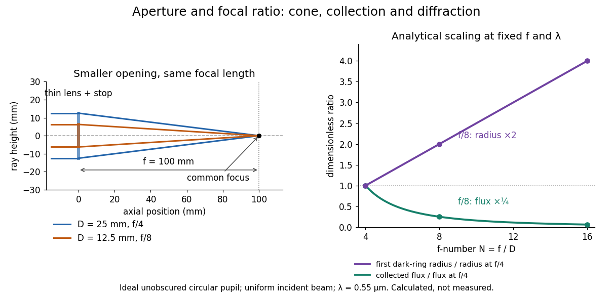
Aperture and focal ratio: a common optical focus, reduced collection and increased diffraction radius
. Original analytical illustration. Left: equal-scale thin lens geometry with and or . Right: collected radiant flux relative to f/4 is , and first-ring radius relative to f/4 is . The wavelength is ; the entrance pupil is circular, uniformly illuminated and unobscured. These are calculated quantities, not measurements. Details.A proposed optical bench check puts a fixed collimator before a converging thin lens and a photodetector large enough to collect the entire image behind it. Compare two centred aperture stops of known diameters while fixing source output, detector gain and integration time. The integrated signal tests the collection law; a spatially resolved optical camera at the focal plane can separately measure the point spread function. Repeat a dark reading and the first aperture stop, and check that neither the incoming beam nor detector clips either bundle. A resolved pinhole source, imperfect collimation, optical aberrations and detector pixel size can dominate the apparent spot width; a single peak reading does not measure total collected radiant flux.
For an initial value problem, convergence means that the largest global error on each fixed finite time interval tends to zero as the step size tends to zero and the starting errors vanish. For linear multistep methods, the Dahlquist equivalence theorem separates this requirement into consistency of a numerical method and zero-stability.
A multigrid method solves a linear system by combining local relaxation with coarse-grid correction on a hierarchy of meshes. The key is to divide the work by scale: a suitable relaxation removes rapidly oscillating approximation error, while coarse-grid correction addresses slowly varying approximation error that relaxation barely changes. A broad error hump occupies many fine-grid points but fewer coarse-grid points; it becomes easier to resolve by relaxation after enough coarsening. This complementary action is why multigrid methods are useful for large finite difference method and finite element method systems.
For a concrete model, take the one-dimensional Poisson equation with homogeneous Dirichlet boundary conditions:Use interior points , , and the centered finite difference systemThus is a symmetric matrix and a positive-definite matrix. The minus sign in fixes this positive convention; changing both and to their negatives leaves the relaxation update unchanged. For , the linear system has the exact discrete solution , since the centered finite difference is exact on this quadratic polynomial. In general, the exact discrete solution need not equal the sampled continuous solution: solving the linear system removes algebraic approximation error, not the global discretization error.
Let solve , let be the current approximation, and define the signed approximation error . The linear-system residual is , so . In particular, a linear-system residual is available without knowing ; it supplies the right-hand side for a correction equation. With , a weighted Jacobi method sweep isThe sine eigenvectors shared by and the iteration matrix are , . Their eigenvalues areFor , one weighted Jacobi method sweep with multiplies the lowest Fourier frequency mode by about , but the highest Fourier frequency mode by about . Four sweeps retain about of the first amplitude and of the second. The sign reversal of the second amplitude is harmless when its magnitude shrinks. However, the plain Jacobi method, , has factor : at it is about . A nearly alternating mode near the grid's Nyquist limit therefore persists almost as strongly as the smoothest mode. Plain Jacobi method convergence on a fixed Dirichlet boundary condition grid does not imply effective smoothing.[ref] The high-frequency smoothing factor of weighted Jacobi is uniformly at most for and ; the exact finite-grid high-frequency Jacobi smoothing optimum distinguishes this convenient uniform choice from the finite-grid optimum.[ref]
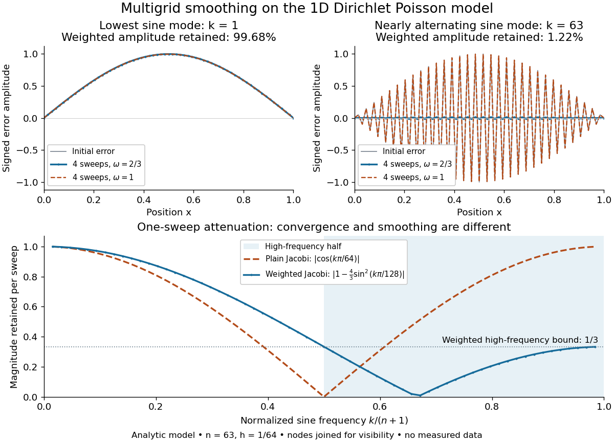
Analytic Poisson error modes: weighted Jacobi damps short wavelengths while plain Jacobi struggles near the Nyquist limit
. Details. One two-grid cycle applies a few weighted Jacobi method sweeps, computes the linear-system residual, performs coarse-grid correction, and applies a few more sweeps. The first relaxation makes the remaining approximation error easier to represent on a coarse mesh; the last relaxation damps oscillatory components left after the transferred correction. In a geometric multigrid V-cycle, replace the expensive exact coarse solve by one recursive cycle on the coarse correction equation, starting its correction from zero. Repeat until a tiny coarsest linear system can be solved directly, then return through the levels by adding each interpolated correction and post-smoothing. The descent and return give the cycle its V shape.[ref]
For this one-dimensional model, fixed sweep counts and bounded local finite difference and transfer work give a geometric multigrid V-cycle cost proportional to , hence in Big O notation. A fixed error reduction also needs a contraction factor bounded below one independently of ; per-cycle work alone does not establish that. Starting from arbitrary approximation error and demanding a relative reduction generally adds a factor proportional to in the cycle count. Full multigrid uses coarse solutions as initial guesses on successively finer meshes to target the global discretization error efficiently. The two-grid Poisson factor with weighted Jacobi illustrates favorable convergence for this model. Other partial differential equations, strong anisotropy, or poorly chosen coarse spaces and relaxation can defeat these choices; a linear-work guarantee for arbitrary linear systems does not follow.
A historical example of the multilevel viewpoint is Achi Brandt's April 1977 paper, which analyzes adaptive meshes and reports numerical experiments on linear and nonlinear boundary value problems. This is a documented development of the approach, not a claim that the paper was its first invention.[ref] The figure above is generated from the displayed eigenvalues, with lines joining discrete nodes; it contains no experimental measurements.
An implicit time-stepping method determines a new solution value through an equation involving that same value. A small-step contraction mapping argument often establishes local solvability when the vector field is Lipschitz continuous. Examples include the Backward Euler method, implicit Runge-Kutta methods and implicit linear multistep methods. Solvability of the update is a separate issue from stability of a numerical method.
The null condition for a nonzero vector in a Lorentzian metric is . Applied to the tangent of a curve it makes the curve a null curve. Nullity alone does not imply the geodesic equation; an additional zero or tangent-parallel covariant acceleration is required.
In Minkowski spacetime with metric signature , write two nonzero future-pointing null vectors as and , where and are unit vectors. Their Lorentzian inner product givesThus their sum is a future-pointing causal vector. It is a null vector exactly when the spatial directions coincide, and a timelike vector otherwise. The positivity of the time components is essential: adding past- and future-pointing null vectors can instead produce a spacelike vector.
Pinned article: Introduction to the OurBigBook Project
Welcome to the OurBigBook Project! Our goal is to create the perfect publishing platform for STEM subjects, and get university-level students to write the best free STEM tutorials ever.
Everyone is welcome to create an account and play with the site: ourbigbook.com/go/register. We belive that students themselves can write amazing tutorials, but teachers are welcome too. You can write about anything you want, it doesn't have to be STEM or even educational. Silly test content is very welcome and you won't be penalized in any way. Just keep it legal!
Intro to OurBigBook
. Source. We have two killer features:
- topics: topics group articles by different users with the same title, e.g. here is the topic for the "Fundamental Theorem of Calculus" ourbigbook.com/go/topic/fundamental-theorem-of-calculusArticles of different users are sorted by upvote within each article page. This feature is a bit like:
- a Wikipedia where each user can have their own version of each article
- a Q&A website like Stack Overflow, where multiple people can give their views on a given topic, and the best ones are sorted by upvote. Except you don't need to wait for someone to ask first, and any topic goes, no matter how narrow or broad
This feature makes it possible for readers to find better explanations of any topic created by other writers. And it allows writers to create an explanation in a place that readers might actually find it.
Figure 1. Screenshot of the "Derivative" topic page. View it live at: ourbigbook.com/go/topic/derivativeVideo 2. OurBigBook Web topics demo. Source. - local editing: you can store all your personal knowledge base content locally in a plaintext markup format that can be edited locally and published either:This way you can be sure that even if OurBigBook.com were to go down one day (which we have no plans to do as it is quite cheap to host!), your content will still be perfectly readable as a static site.
- to OurBigBook.com to get awesome multi-user features like topics and likes
- as HTML files to a static website, which you can host yourself for free on many external providers like GitHub Pages, and remain in full control

Figure 2. You can publish local OurBigBook lightweight markup files to either OurBigBook.com or as a static website.
Figure 3. Visual Studio Code extension installation.
Figure 5. . You can also edit articles on the Web editor without installing anything locally. Video 3. Edit locally and publish demo. Source. This shows editing OurBigBook Markup and publishing it using the Visual Studio Code extension. 
- Infinitely deep tables of contents:




All our software is open source and hosted at: github.com/ourbigbook/ourbigbook
Further documentation can be found at: docs.ourbigbook.com
Feel free to reach our to us for any help or suggestions: docs.ourbigbook.com/#contact