
Twist-spun knot Created 2026-09-24 Updated 2026-10-14
Arf invariant of a knot Created 2026-09-24 Updated 2026-10-14
The Arf invariant is a -valued concordance invariant obtained from the quadratic refinement of the mod-two intersection form on a Seifert surface.
Amphichiral knot Created 2026-09-24 Updated 2026-10-03
An amphichiral knot is ambient-isotopic to its mirror. Positive and negative amphichirality distinguish whether the symmetry preserves or reverses the knot orientation.
Two-fold branched cover of a knot Created 2026-09-24 Updated 2026-10-14
The two-fold branched cover of a knot is the double cover of branched along the knot. Its first homology has a nonsingular linking form and, when finite, has order .
Away from the knot this is a two-sheeted covering space; at the knot it has the standard local model of a branched covering.
Knot concordance Created 2026-09-24 Updated 2026-09-24
Two knots are concordant when they cobound a smoothly embedded annulus in . Connected sum makes concordance classes into an abelian group.
Knot Created 2026-09-24 Updated 2026-10-14
A knot is the image of a smooth embedding , considered up to ambient isotopy. The circle supplies a closed loop with no free ends; the smooth embedding condition rules out self-intersections and requires a nonzero tangent vector in a regular parametrization. The equivalent convention uses the three-sphere: removing a point outside the knot identifies the remaining space with three-dimensional Euclidean space by stereographic projection.
More precisely, knots are equivalent if there is a smooth family of diffeomorphisms of the ambient space, for , such that is the identity and . Every intermediate remains a smooth embedding. This ambient isotopy allows bending, stretching and moving a loop, but neither cutting it nor letting strands cross through each other. We compare the embedded images rather than their parametrizations; an oriented knot additionally remembers a direction of travel.
For a worked example, start with , where is taken modulo , and useBoth scale factors stay positive, so each is a diffeomorphism. At the circle becomes the ellipse , yet its knot type is still the unknot. Exact lengths and angles are therefore irrelevant to knot type; self-intersection is the obstruction that the deformation must avoid.
Linearized boundary condition Created 2026-09-24 Updated 2026-09-24
For a small boundary displacement and weak disturbance, evaluate boundary data on the undisturbed surface and discard products of small quantities.
Kinematic boundary condition for a free-surface graph Created 2026-09-24 Updated 2026-11-05
Geodesic conserved quantity from a Killing vector Created 2026-09-24 Updated 2026-10-14
Each Killing vector field supplies a conserved quantity for freely moving test particles: it turns a geometric symmetry into a first integral of the geodesic equation. Let be a geodesic with affine parameter , tangent vector , and . Wherever a Killing vector field is defined along the geodesic,The statement applies to Riemannian manifolds and to timelike geodesics, null geodesics and spacelike geodesics in a Lorentzian manifold. It requires an affine parameter; for a massive test particle, proper time is one choice. See Tong, section 4.3.2, equation (4.32).
For a worked example in the Euclidean plane, take with affine parameter and velocity . The Euclidean Killing vector fields for translation and rotation giveThe rotational field along the geodesic is : it changes from at to at , yet its pairing with stays . With toy mass and interpreted as time, the first constant is the component of linear momentum, and the second is the signed component of angular momentum about the origin. Their numerical values use toy units. The geodesic is straight; the rotation flow orbits are circles.
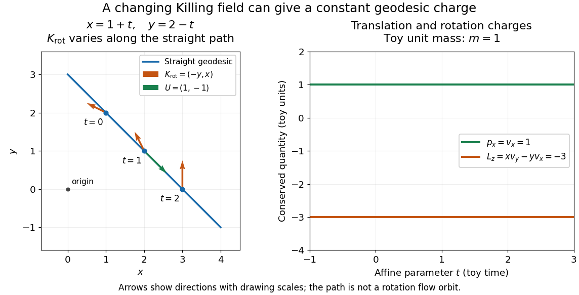
One straight Euclidean geodesic: the rotational Killing field varies while translation momentum and angular momentum stay constant for toy unit mass
. Details. 
This conservation law follows from metric compatibility and the Killing equation:The geodesic equation kills the acceleration term, and the symmetric product selects the vanishing symmetric derivative. This tensor contraction is the whole proof outline; see Carroll, equation (5.43).
In a stationary spacetime, a chosen time-translation Killing vector field gives Killing energy. With metric signature , , and a massive test particle's four-momentum , the physical normalization isHere generates the axial rotational symmetry when one exists. In coordinates with and , these are and . Both are conserved quantities along the geodesic, even if the metric has a time-angle cross term. A future timelike makes positive for a future massive particle; the scale of depends on the normalization of . Not every spacetime has a global timelike Killing vector field, and a stationary field can become spacelike in an ergoregion of a stationary spacetime. Conservation on the field's domain does not imply a universal global positive energy; see Tong, sections 4.3.1-4.3.2 on the timelike-domain qualification and conserved charges.
Active-set transition in capped resource allocation Created 2026-09-24 Updated 2026-10-14
Discrete scattering data Created 2026-09-24 Updated 2026-10-14
Discrete scattering data consist of the discrete eigenvalues and norming constants associated with bound states of the auxiliary spectral problem. Their simple time evolution reconstructs solitons and breathers through the inverse problem.
Mountain-wave cutoff Created 2026-09-24 Updated 2026-11-05
For a stationary topographic internal gravity wave in a uniform horizontal velocity and constant buoyancy frequency , a nonzero horizontal wavenumber gives intrinsic frequency . The nonrotating Boussinesq approximation givesVertical propagation therefore requires . At , the vertical wavenumber vanishes and so does the vertical group velocity; this grazing limit carries no finite upward energy flux for a finite-amplitude plane mode. For , the vertical wavenumber is imaginary and the bounded response is an evanescent wave. A hill pattern with very short horizontal wavelength can consequently produce a local disturbance without radiating an upward internal gravity wave.
Vertical trapping of an internal gravity wave by planar strain Created 2026-09-24 Updated 2026-11-05
Consider nonrotating internal gravity waves in constant buoyancy frequency and the imposed planar strain-rate tensor corresponding to , with . The internal-wave ray tracing equations advect the horizontal and vertical wavenumbers asFor , and initial height , the intrinsic vertical group velocity is . Including mean advection givesEvery term in the bracket is positive. Moreover, , so the bracket tends to a positive finite limit. Thus the ray remains above at finite time and approaches it as , despite its upward intrinsic group velocity. This is a ray prediction within the imposed flow with density stratification, rather than a statement that a finite-amplitude beam can contract indefinitely without viscous attenuation of an internal-wave beam.
Buoyancy frequency Created 2026-09-24 Updated 2026-11-05
The buoyancy frequency is the natural angular frequency of a small vertical parcel displacement in a stably stratified fluid. In an incompressible Boussinesq model, with height upward and background mass density ,A parcel lifted into lighter surroundings is too dense for its new position, so buoyancy accelerates it downward. Positive gives oscillation; negative gives a growing displacement in this ideal local model.
A tank with denser salt water below fresher water provides a physical example. Gently displacing a small neutrally buoyant object or marked parcel reveals the restoring tendency, although drag and diffusion modify the measured motion. In a compressible atmosphere the parcel changes density adiabatically as it moves, so the stability formula must compare its response with the ambient stratification rather than simply reuse the incompressible density gradient.
Square-free integer Created 2026-09-24 Updated 2026-11-05
A positive integer is square-free when no square number greater than one is a divisor of . It suffices to exclude squares of prime numbers; equivalently, every prime valuation is zero or one:Thus the prime factorization of a square-free integer is a product of distinct prime factors, with no repetitions. One is included: its prime factorization is an empty product and all its prime valuations are zero. These equivalent tests are stated in Grinberg's notes. [ref]
Floor and arithmetic functions by Darij Grinberg. Darij Grinberg, MIT 18.781, Floor and arithmetic functions, Definition 2.1.2 and footnote 6
For signed integers, extend the definition by requiring to be a square-free integer, where denotes absolute value. Hence and both qualify. Zero does not: every prime number has its square as a divisor of zero. The Möbius function and radical of an integer below use their existing positive integer domains, so apply them to when handling a negative integer.
For example, is a square-free integer, whereas is not, because and . Being a composite number causes no problem: are all square-free integers. A square-free integer need not be coprime to another integer: and are both square-free integers but have greatest common divisor two. In fact the only signed integers coprime to every integer are , since .
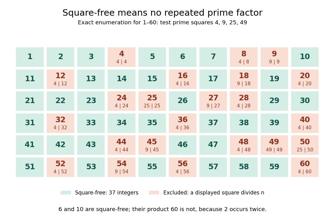
Exact square-free integer classification of the integers from one to sixty
. Green cells are square-free integers; each red cell displays a prime number square that divides its label, choosing the smallest such prime number. Only need testing in this range. There are green cells. This original finite arithmetic diagram is an exact enumeration, not a measurement or an assertion about a limiting frequency. Details.
For positive integers , the useful product criterion isThe proof outline is just addition of prime valuations: can stay at most one only if neither input repeats a prime factor and no prime factor occurs in both. Thus is a square-free integer, but is not. An equivalent characterization is that every factorization into positive integers has coprime factors. If , the factorization supplies two factors sharing ; conversely, a shared prime factor forces its square to divide . For , the unordered factor pairs all have greatest common divisor one; for , the pair fails.
Two existing arithmetic functions turn the definition into practical tests:The radical of an integer keeps one copy of each prime factor, so it changes precisely the integers with a repeated prime factor. Its definition is given in Evertse's exercise sheet. [ref]
https://pub.math.leidenuniv.nl/~evertsejh/dio12-ex4.pdf. Jan-Hendrik Evertse, Diophantine approximation, Homework IV, Exercise 20
The Möbius function assigns to a square-free integer with distinct prime factors and zero otherwise; squaring forgets the sign. Consequently counts exactly the green cells. This connects a restriction on repeated prime factors with weighted counting and inclusion-exclusion. [ref]Floor and arithmetic functions by Darij Grinberg. Darij Grinberg, MIT 18.781, Definition 2.1.2: the Möbius function
Odd number Created 2026-09-24 Updated 2026-11-05
An odd number is an integer not divisible by . Equivalently, it has the unique formThe Euclidean division remainder is one. Examples include ; zero is excluded because it is an even number. The property is independent of primality: is a prime number, is a composite number, and is neither.
Even number Created 2026-09-24 Updated 2026-11-05
An even number is an integer divisible by , so it has the form for an integer . Examples include ; zero is even because . This is the zero remainder class in Euclidean division by .
The only prime number that is even is . Every greater positive even integer has as a proper divisor. This explains why many primality testing procedures handle separately before discarding other even inputs.
Positive integer Created 2026-09-24 Updated 2026-11-05
Unicity distance Created 2026-09-24 Updated 2026-11-05
Unicity distance is the ciphertext-length scale at which a specified cipher and plaintext model are expected to leave essentially one plausible cryptographic key. Claude Shannon obtained an approximate threshold from the sharp decrease of key equivocation in a random-cipher model; it is not a universal length guaranteeing zero residual conditional entropy for every ciphertext.[ref]
Communication Theory of Secrecy Systems by Claude Shannon. Sections 14–15, printed pp. 691–695, especially the discussion after Figure 7
For a realized ciphertext, uniqueness depends on which candidate decryptions the plaintext model allows. A probability distribution giving every finite plaintext positive mass need not exclude every wrong cryptographic key at any finite length. A source symmetry can even preserve ambiguity forever. The source redundancy in cryptanalysis estimate therefore needs its source and cipher assumptions.
Asymptotic equipartition property Created 2026-09-24 Updated 2026-10-14
The asymptotic equipartition property explains why a long message from a source can usually be described using its information entropy per symbol. Individual messages can have very different probabilities, but the messages carrying almost all the total probability have similar logarithmic costs per symbol. The Bernoulli typical-set example makes the distinction between an individual message and a large collection explicit.
For independent and identically distributed random variables on a finite alphabet, let be their probability mass function and . ThenHere means the probability mass of the realized word, evaluated under the source law. The product rule for independent random variables turns its information content into a sum:The strong law of large numbers gives the limit. Zero-probability symbols do not occur; on the positive-probability support of a finite alphabet, these information costs are finite. The corresponding typical set consists of words whose cost per symbol is within a chosen tolerance of .
For a strictly stationary process with a finite alphabet, the constant-limit extension requires ergodicity. The Shannon-McMillan-Breiman theorem then replaces the one-symbol information entropy with the information rate. Stationarity without ergodicity in an information source shows why stationarity alone is insufficient.[ref]
6.441 Information Theory (Spring 2016 lecture notes) by Yury Polyanskiy and others. §8, Theorem 8.1 and Corollary 8.2, printed p. 90: stationary ergodic sources and typical sets
There are unlisted articles, also show them or only show them.