
Unimodular matrix Created 2026-09-24 Updated 2026-10-14
A unimodular matrix is a square integer matrix whose determinant is or . The decisive property is that its inverse matrix also has integer entries: multiplication by gives a bijection of the integer lattice onto itself. Thus an invertible linear map can preserve not only real coordinates but the requirement that every coordinate is an integer. These matrices form the integral general linear group.[ref]
Lecture 1: Introduction. §7, Definition 11 and Lemma 12, printed p. 9: determinant and integer-inverse characterization
For an original two-dimensional example, takeIts determinant is one, and it maps to . Conversely, the integer point comes from . For instance, has new coordinates relative to the columns and . No integer point disappears, although the basis vectors and their fundamental cell change shape.
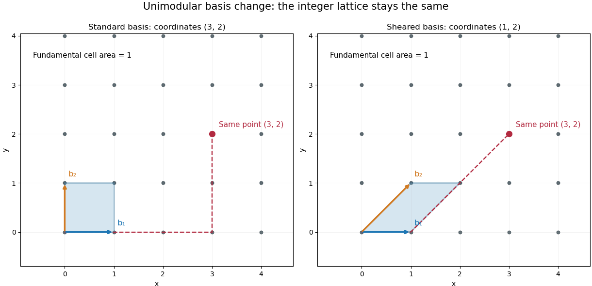
Two lattice bases generate exactly the same integer points
. Original drawings of the standard basis and the columns of . Both displayed cells have area one. The point has coordinates in the standard basis and in the sheared basis. Details.This is useful whenever coordinates must remain integral. A unimodular change of lattice basis can give a shorter or more convenient description without changing the objects represented. Smith normal form and Hermite normal form use controlled integer operations to simplify integer matrices; ordinary Gaussian elimination may divide by numbers that destroy integrality. The geometric freedom is substantial: a sheared basis may look completely different while describing exactly the same infinite set of integer points.
A determinant of is allowed too. Swapping two basis columns reverses orientation while preserving the integer lattice. The condition is therefore preservation of the complete integer structure, rather than a requirement to preserve orientation.
Singular value decomposition Created 2026-09-24 Updated 2026-10-14
The singular value decomposition separates any matrix into input directions, stretching factors, and output directions. Every complex matrix admitsHere are unitary matrices, is the conjugate transpose, and is a rectangular diagonal matrix. Its diagonal entries are the singular values, ordered . We use the conventional letters: contains the right singular vectors , while contains the left singular vectors . Writing instead merely swaps these two matrix names; it requires swapping their roles consistently. For real matrices, choose orthogonal matrices and replace the conjugate transpose with the transpose.[ref]
Reading from right to left, expresses the input in an orthonormal basis, stretches or annihilates those coordinates, and assembles the output in another orthonormal basis. Unlike matrix similarity, the input and output bases can differ, and even have different sizes. A matrix has full factors of sizes , , and . If its matrix rank is , one can retain only the active columns, giving sizes , , and for ; the full additionally describes an unused output direction.
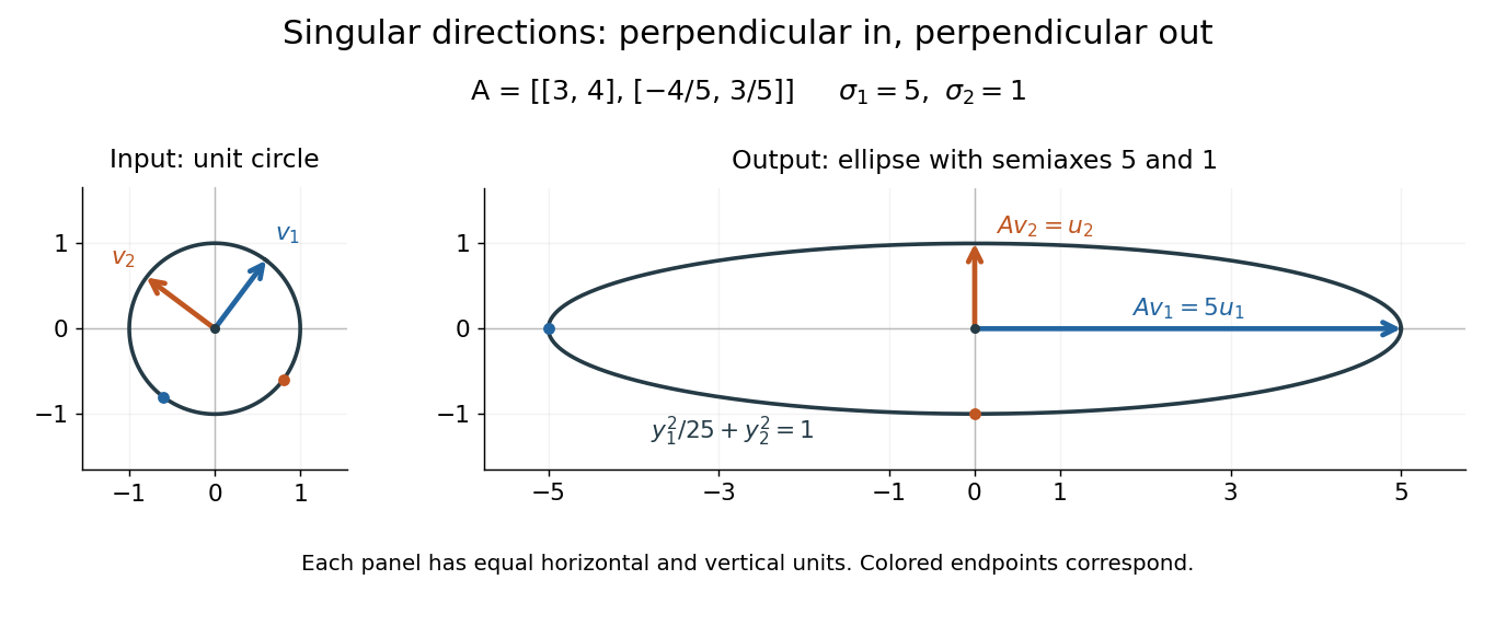
For a fully computed nonsymmetric example, takeMultiplication gives . The right singular vectors are and ; their images are and . Thus, parametrizing the unit circle by gives . Its image is the ellipse . The two singular values are its semiaxis lengths, and the left singular vectors point along its axes. The singular value decomposition finds precisely the perpendicular input directions whose images stay perpendicular.
For compression, write the matrix as a sum of outer products and retain the largest terms:where is the matrix rank. Among all matrices of matrix rank at most , minimizes the Frobenius norm error; this is the Eckart-Young-Mirsky theorem. The operator norm error is for . These statements concern specified norms, rather than guaranteeing that discarded details are visually or scientifically unimportant.[ref]
Consider an brightness matrix , withand , . The broad bright patch and alternating checkerboard have orthogonal row and column directions: . Their singular values are and . This low-rank approximation keeps the first outer product, giving , with Frobenius norm error and relative error . For example, becomes , and becomes : every entry changes by in magnitude. The discarded pattern is small but entirely lost.
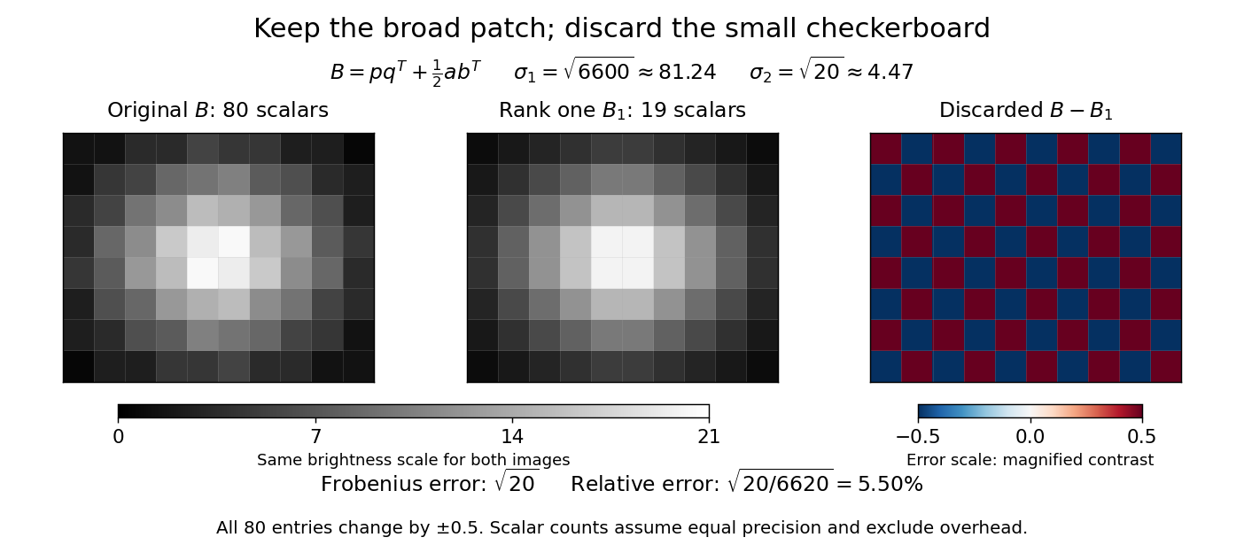
For this illustrative image compression, storing one normalized left singular vector, one normalized right singular vector, and one singular value requires scalars instead of . This counts scalars at equal precision, before storage overhead. In general, scalars beat only for sufficiently small , and small error requires a small discarded sum of squared singular values. The usefulness comes from measuring the tradeoff before throwing information away.[ref]
https://math.mit.edu/~gs/linearalgebra/ila5/SVD_Slides.pdf. Verma, Singular value decomposition of real matrices, slides 9 and 15–16
Vector space Created 2026-09-24 Updated 2026-10-14
A vector space over a field is a set equipped with vector addition and scalar multiplication satisfying the vector space axioms. Its vectors can represent directed displacements, lists of measurements, polynomials, or entire functions. The common structure is that adding two elements and multiplying an element by a scalar remain meaningful operations inside the same space.
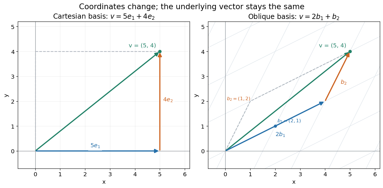
For example, uses coordinatewise addition and scaling. Withwe have . Moving twice along and once along reaches the same vector as five horizontal and four vertical steps. The two descriptions refer to different bases of the same space. A basis makes such descriptions unique; a spanning set makes them possible.


The space of real polynomials of degree at most two has basis : the polynomial is the linear combination with coordinates . The zero vector here is the zero polynomial, and addition combines coefficients. A derivative is a linear map on this space; its matrix records how it acts on the three basis vectors. The same coordinate machinery therefore handles both geometric motion and operations on functions.
The choice of field matters. The complex numbers form a one-dimensional vector space over with basis , but a two-dimensional vector space over with basis . The question "how many independent directions?" has an answer only after the allowed scalars are specified. Likewise, polynomials of degree exactly two do not form a vector space: subtraction can remove the leading term, and the zero polynomial is absent.
The usefulness of the abstraction is that a linear map is determined by its values on a basis. Once those images are known, linear combinations give its action on every vector. The rank-nullity theorem relates the number of attainable outputs to the number of invisible input directions, while change of basis lets us choose coordinates suited to the problem. Eigenvectors, for example, choose directions on which repeated application of a linear operator becomes scalar multiplication.
A historical source is Hermann Grassmann's Die lineale Ausdehnungslehre (1844). Its full title advertises applications to other branches of mathematics, statics, mechanics, magnetism and crystallography; the original edition is digitized by ETH-Bibliothek. This gives an early setting for treating geometric quantities algebraically across different applications, rather than attributing the modern axiom list to that title alone.[ref]
https://www.e-rara.ch/zut/content/titleinfo/1169335. Grassmann, Die lineale Ausdehnungslehre, Leipzig, 1844; ETH-Bibliothek Rar 5128
Sesquilinear form Created 2026-09-24 Updated 2026-10-14
A sesquilinear form on a complex vector space is a map which, with the convention used throughout this article, is a linear map in its first argument and a conjugate-linear map in its second. For vectors and complex numbers , the defining identities areThe bars denote complex conjugation. No symmetry or positivity is required. Some authors choose the opposite convention; every formula here keeps the first argument linear.[ref]
For a basis of a finite-dimensional vector space, write , , and . Expanding by the two identities givesEvery complex matrix gives a sesquilinear form this way. The superscript means transpose, not conjugate transpose. Equivalently, the scalar is , where . This is the convention used for the matrix of a Hermitian form when symmetry is imposed. The coordinate formula follows directly by expanding the basis coefficients.[ref]
https://sites.math.washington.edu/~burke/crs/554/lectures/b-lecture4.pdf. Burke, Linear Analysis, Lecture 4, coordinate expansion for sesquilinear forms
For a concrete example on , let . Its matrix is : but , so it is not a Hermitian form. Also , so even real diagonal values cannot be assumed for an arbitrary sesquilinear form. By comparison, the bilinear form satisfies and has ; it cannot supply positive squared lengths on this complex vector space.
The effect of changing the complex argument of a multiplier is particularly revealing. For real numbers , sesquilinear forms satisfyThus a common change of complex argument cancels from the diagonal, whereas the two arguments rotate the output in opposite directions. Conjugating one argument is what replaces the scaling of a bilinear form by the nonnegative scaling needed for a Hermitian inner product. This mechanism also works in function spaces: for complex continuous functions on , obeys the same identities, letting integration measure overlap rather than merely multiply coefficients.
Bilinear form Created 2026-09-24 Updated 2026-10-14
A bilinear form takes two vectors in a vector space over a field and returns a scalar in . Its defining property is separate linearity: holding either input fixed gives a linear functional of the other. For scalars and vectors ,This is a scalar-valued bilinear map; the chosen field is part of the definition.[ref]
Separate linearity does not mean that is a linear map on the vector space with componentwise vector addition and scalar multiplication. Over the real numbers, , whereas a linear map on the pair would give . The simplest example is on the one-dimensional vector space : fixing gives , but doubling both and quadruples their product.
A bilinear form measures how two inputs interact. The dot product measures alignment; a symmetric bilinear form can describe a quadratic form; an alternating bilinear form can measure signed area. A nondegenerate bilinear form turns each vector into a unique linear functional and so connects geometry with the dual space. The same short definition therefore supports lengths, bilinear orthogonal complements, and symplectic vector spaces, depending on the additional properties imposed.
Over the complex numbers, a bilinear form is linear in both inputs without conjugating either scalar. A Hermitian form instead is a sesquilinear form and conjugates when its inputs are exchanged. For complex matrices, the adjoint used with Hermitian forms and matrix C-star algebras is the conjugate transpose, whereas a bilinear form uses the ordinary transpose . For example, has , while the Hermitian form has .[ref]
Bilinear Forms by Keith Conrad. §1: examples and the Hermitian distinction
Cartesian basis Created 2026-09-24 Updated 2026-10-14
A Cartesian basis is an ordered basis of unit vectors along the mutually perpendicular axes of a Cartesian coordinate system. It is an orthonormal basis of a real Euclidean space: , with the Kronecker delta. In the plane, the familiar standard basis is , ; the vector is . A rotated pair of perpendicular unit vectors is also a Cartesian basis, even though its basis vectors have different standard basis entries.
The advantage is that coordinates can be measured separately by dot products, and the squared norm is the sum of their squares:These are the real Euclidean space instances of the orthonormal basis expansion.[ref]
Linear Algebra Done Right by Sheldon Axler (4th edition). §6B, Definition 6.27, printed p. 199, and Theorem 6.30(a–b), printed p. 200
An orthogonal basis only requires perpendicular basis vectors; their lengths need not be one. For example, are orthogonal, but has coordinates , while its dot products with them are . For an orthogonal basis , the coordinate along is . Dividing each nonzero basis vector by its norm makes it a unit vector without changing its direction. Unit length alone does not imply orthogonality: and are both unit vectors but have dot product .
The examples below show why these distinctions matter: rotating a Cartesian basis changes the coordinate vector while keeping lengths easy to compute; using nonperpendicular basis vectors still gives unique coordinates, but requires the dual basis or a matrix inverse to extract them.
Time average of harmonic power Created 2026-09-24 Updated 2026-09-24
Evanescent acoustic surface wave Created 2026-09-24 Updated 2026-09-24
Acoustic energy conservation Created 2026-09-24 Updated 2026-09-24
Acoustic velocity potential Created 2026-09-24 Updated 2026-10-03
Homentropic pressure perturbation Created 2026-09-24 Updated 2026-09-29
Singular Legendre transform of a degree-one velocity Lagrangian Created 2026-09-24 Updated 2026-11-05
For positive constants and nonzero velocity , consider the Lagrangian . Its canonical momentum and canonical energy areThe canonical momentum records direction but loses speed: every positive rescaling of gives the same . Its velocity Hessian matrix is , where . It has the velocity direction in its kernel, so the Lagrangian is not a regular Lagrangian and has no ordinary inverse Legendre transform in mechanics.
The expression is an energy value on the constraint surface , not an unconstrained Hamiltonian describing all positions and momenta. Using it alone in ordinary Hamilton's equations would wrongly set the velocity to zero. A constrained Hamiltonian treatment must enforce the momentum relation and its consistency with the chosen . For constant , the Euler-Lagrange equations keep the direction fixed while leaving the positive speed along the path undetermined; that freedom is exactly the information the momentum map lost.
Global relation for the half-line free Schrodinger equation Created 2026-09-24 Updated 2026-09-24
For on , the half-line Fourier transform satisfiesSubtracting the relation at cancels the unknown Neumann datum. Fourier inversion of the resulting odd combination gives the solution in terms of the initial transform and the prescribed Dirichlet datum, with boundary kernel .
Zero-curvature condition Created 2026-09-24 Updated 2026-10-14
For and , compatibility is .
For the auxiliary equations and , equality of mixed derivatives gives . This is the compatibility condition for a Lax pair.
Isospectral Lax equation Created 2026-09-24 Updated 2026-10-03
AKNS Lax pair for the nonlinear Schrodinger equation Created 2026-09-24 Updated 2026-09-24
For complex fields , the standard two-by-two AKNS pair has zero-curvature equationsThe reductions and give the focusing and defocusing cubic nonlinear Schrödinger equations, respectively.
Airy equation Created 2026-09-24 Updated 2026-10-14
The Airy equation is the linear dispersive partial differential equation . Under the spatial Fourier transform, each mode evolves by multiplication by .
For positive time its fundamental solution is , connecting this evolution equation to the Airy function without identifying the two concepts.
Laurent theorem Created 2026-09-24 Updated 2026-10-31
An analytic function on an annulus has a unique locally uniformly convergent expansionwhere is any positively oriented circle around in the annulus.
Dyck path Created 2026-09-24 Updated 2026-10-14
A Dyck path starts at , ends at , uses steps and , and never passes below the horizontal axis. Its semilength of a Dyck path is : there are up steps and down steps. The nonnegative height records a constraint throughout the journey, not just the endpoint. The Catalan number counts the Dyck paths of this size.
Soft thresholding Created 2026-09-24 Updated 2026-10-03
There are unlisted articles, also show them or only show them.