
Bernoulli source Created 2026-09-24 Updated 2026-09-24
Huffman coding Created 2026-09-24 Updated 2026-10-14
Huffman coding makes frequent symbols cheap to store by giving them short codewords, while allowing rare symbols longer codewords. For a known probability distribution on a finite alphabet with at least two positive-probability symbols, binary Huffman coding constructs a prefix code minimizing expected codeword length among binary prefix codes that encode one source symbol at a time. The objective is an average under that probability distribution; it does not promise to shorten every message. Encoder and decoder must agree on the resulting Huffman code. [ref]
The construction grows a binary tree from its leaves towards its root of a tree. Start with one leaf per symbol, weighted by its probability. Repeatedly join the two currently smallest weights beneath a new parent in a rooted tree, whose weight is their sum, and replace the pair by that subtree. Include newly formed subtrees when choosing the next pair. When one tree remains, label the two outgoing edges at every internal vertex with and ; the labels on the graph path from the root of a tree to a symbol give its codeword. This is a greedy algorithm: each step makes a locally cheapest merge, yet the result is an optimal prefix code.
For a concrete example, use probabilities , , , . First join and , creating weight . The remaining weights are for , for the subtree, and for . Join the two weights to make , then join with that subtree to make . The merge weights are therefore . Each merge adds one bit to every codeword below it, so their sum is the expected codeword length: bits per source symbol. The diagram fixes the edge labels to produce the Huffman code used below.
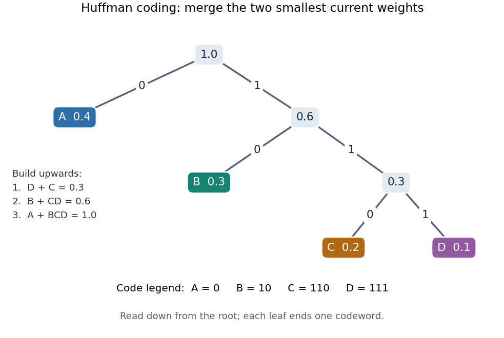

The useful insight is that choosing short codewords is a resource allocation problem: the prefix code condition constrains the available codeword lengths through the Kraft inequality. Huffman coding solves this one-symbol problem exactly for the supplied probability distribution. For repeated emissions of a memoryless classical information source, the same Huffman code can be applied symbol by symbol. More general compression can exploit dependencies or encode groups of symbols; the one-symbol optimality statement does not compare all such methods.
One-to-one source code Created 2026-09-24 Updated 2026-09-24
A one-to-one source code is an injective function from source symbols to finite codewords. Unlike a prefix code, it need not permit instantaneous decoding of concatenated codewords.
Information entropy Created 2026-09-24 Updated 2026-10-14
For a finite discrete random variable with probability mass function , its information entropy is the expected value of its information content:Base-two logarithms give bits; choosing a different base rescales the units. The convention is justified by a limit, so outcomes of zero probability contribute nothing. The definition also applies to countable distributions, but the sum may be infinite.
A fair bit has . A certain outcome has . A Bernoulli random variable that is one with probability has bits, because most of its outcomes are predictable. A rare outcome still has large information content: the outcome of probability contributes bits of surprise when it occurs. Entropy is the average surprise, rather than the surprise of each outcome.
For possible outcomes, , with the upper bound attained exactly by the uniform distribution on a finite set. The Gibbs inequality proves this by comparing with the uniform distribution: . Thus increasing predictability reduces the required average description length. The four-symbol prefix code in information theory attains bits exactly; for general probabilities, integer codeword lengths prevent such a perfect match for every individual symbol. Shannon's source coding theorem explains how coding sufficiently long independent blocks approaches the entropy per symbol.
The logarithm is especially natural because independent outcomes have additive surprise: . Taking expected values gives additive information entropy for independent random variables; for dependent ones, the chain rule for information entropy replaces the second term by conditional entropy. This is why the same quantity can govern both a single observation and a long message.
Channel capacity Created 2026-09-24 Updated 2026-10-14
Channel capacity is the best reliable information rate available through a specified communication channel. For a discrete memoryless channel with finite input and output alphabets, fixed transition probabilities , and no input-cost constraint, it isin bits per channel use, when the mutual information uses base-two logarithms. The maximization varies the input probability distribution, while keeping the communication channel fixed. A large input alphabet or a large output information entropy alone does not determine how much information gets through: the receiver needs information about the input, rather than merely unpredictable output.
The operational meaning comes from the Shannon second coding theorem. A block code represents one of possible messages by a word of length , giving a rate bits per use. Take the message label from the uniform distribution on a finite set of those choices when measuring average decoding-error probability. For every fixed rate , there are sequences of such block codes whose decoding-error probability tends to zero as grows; a rate above cannot have vanishing decoding-error probability. This is an asymptotic limit, rather than a promise that an arbitrary finite block code at a rate below works well. See MIT 18.310, Shannon's Noisy Coding Theorem, sections 1–2.
For a binary symmetric channel with crossover probability , the binary symmetric channel capacity is approximately bits per use. Thus a binary code rate lies below the limit, while lies above it. At , two transmitted symbols represent one message bit on average; the redundancy helps distinguish messages after noise. This does not split individual physical symbols into fractional pieces.
The result is useful because it separates two tasks. Computing channel capacity establishes the target imposed by the transition probabilities; constructing an effective block code attempts to approach that target with acceptable delay and decoding effort. The surprise is that reliability can improve indefinitely without forcing every positive rate to disappear. In his 1948 paper, Shannon defines noisy channel capacity in section 12 and develops its operational significance in section 13, Theorem 11. His original formulation uses information per unit time; the fixed-duration channel-use convention here expresses the same rate question per symbol. [ref].
Type (information theory) Created 2026-09-24 Updated 2026-10-14
A type summarizes a string by how often each symbol occurs. Fix a finite alphabet of cardinality and a positive length . For a string , its empirical distribution is the probability mass functionThe empirical distribution forgets order. The strings and both assign probability to each binary symbol; assigns to zero and to one. Thus a long string can have a short summary even though that summary does not reconstruct the original order.
For independent and identically distributed symbols, this loss of order has a useful consequence: all strings with the same empirical distribution have the same probability. The method of types uses this symmetry to turn questions about exponentially many strings into counting questions about relatively few frequency profiles.[ref]
The Method of Types by Imre Csiszár. §I, printed p. 2505: partition by empirical distribution and equiprobability under a memoryless model
Binary hypothesis testing in information theory Created 2026-09-24 Updated 2026-09-24
For two probability mass functions , a decision region accepts . Its two error probabilities are and .
Entropy submodularity for three independent sums Created 2026-09-24 Updated 2026-09-24
For independent finitely supported random variables in a finite additive group,This is the data processing inequality for mutual information applied to the Markov chain .
Entropic Ruzsa distance Created 2026-09-24 Updated 2026-09-24
For finitely supported random variables in a finite additive group, let be independent variables with their respective marginal distributions. The entropic Ruzsa distance isIt is symmetric and nonnegative, but can have .
Mutual information Created 2026-09-24 Updated 2026-10-14
For finite discrete random variables, mutual information is the reduction of information entropy provided by observing the other variable:The last expression makes the symmetry visible. It is nonnegative and is zero exactly when and are independent random variables. One way to see both facts iswhere is the Kullback-Leibler divergence with base-two logarithms. The Gibbs inequality gives nonnegativity; equality means that the joint probability distribution factors. The statement extends to more general distributions via relative entropy, but differences of infinite information entropies must not be used as if they were finite numbers.
A binary symmetric channel gives a useful example. Let be a fair bit, let be an independent Bernoulli random variable with error probability , and set , where is exclusive or. The output is also a fair bit, but knowing the input leaves just the error uncertainty:Here is binary entropy. At , , so the output carries about bits of mutual information about the input per use. This is an average uncertainty reduction, not a claim that each observed symbol can be divided into fractional physical bits.
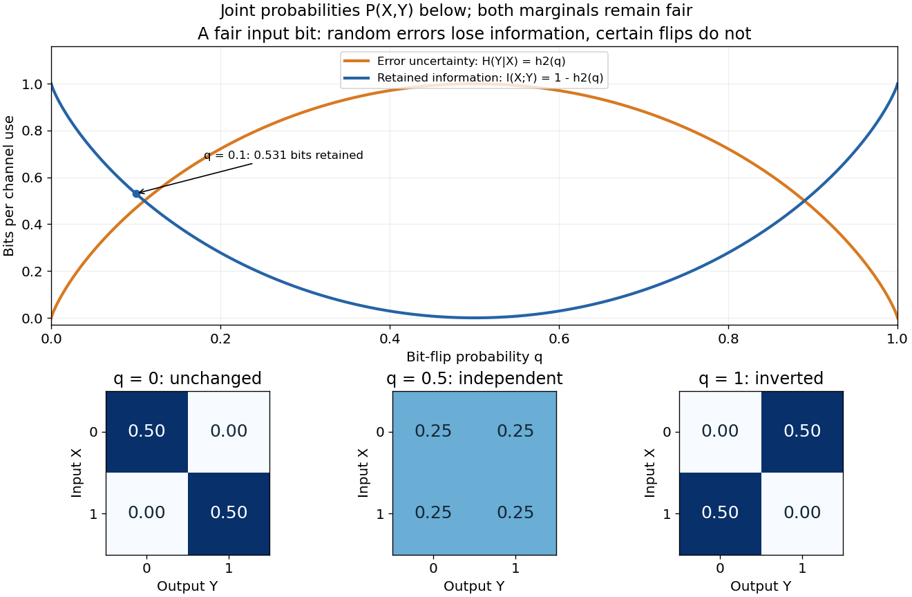
Binary entropy and retained information distinguish noisy transmission from predictable bit inversion
. Details. 
At , every output is equally likely for either input, so . At , the output is always the inverted input: knowing this rule lets the receiver recover the input exactly, so again. A high raw error rate need not mean low mutual information when the errors are predictable. For this particular channel the fair input is optimal, giving the binary symmetric channel capacity .
Mutual information detects dependence that ordinary correlation can miss. Let be uniform on and . Symmetry gives , hence zero covariance and zero correlation, while is completely determined by . Thus . This distinction is useful whenever a relationship is nonlinear: knowing one variable can reveal another without a linear trend.
Conditional entropy Created 2026-09-24 Updated 2026-10-14
For finite discrete random variables, conditional entropy is the average remaining information entropy of after the value of is known:Each observation changes the probability distribution used to describe ; the average weights that uncertainty by how often the observation occurs. An observation can increase uncertainty for one particular outcome, even though conditioning reduces entropy on average for finite variables.
For example, let choose with probabilities , and let report whether . If it reports yes, there is no remaining uncertainty. Otherwise the conditional probabilities are , whose information entropy is bits. The two reports each occur with probability , so of a bit. The original uncertainty was bits: this observation removes exactly one bit on average.
If is a function of , then : the observation determines the answer. If and are independent random variables, then : the observation gives no improvement. These endpoints make conditional entropy useful for separating relevant observations from irrelevant ones. They also lead to the chain rule for information entropy, , which counts the first uncertainty and the remaining uncertainty without double counting.
Alphabet Created 2026-09-24 Updated 2026-10-14
Particle in a rectangular box Created 2026-09-24 Updated 2026-11-05
A particle of mass confined by infinite walls to , , has Dirichlet boundary conditions. Separation of variables gives the normalized product energy eigenstatesEach factor comes from the infinite square well, and its second derivative contributes one term to the kinetic energy. The minimum uses ; zero quantum numbers would give the zero wavefunction, not a lower energy state.
For a cube, permuting unequal quantum numbers can produce degenerate energy levels. The first excited energy has the three basis states , and , each with . A general state in that eigenspace is a linear combination of those products, so degeneracy permits stationary states that are not a single separated product.
Divergence-free vector field Created 2026-09-24 Updated 2026-11-05
Endpoint expansion of the incomplete gamma function Created 2026-09-24 Updated 2026-11-05
For a fixed and real , the upper incomplete gamma function has leading endpoint approximationSet in its defining integral:The phase is increasing for , with derivative at the endpoint. The leading endpoint form of Laplace's method gives amplitude divided by , proving the formula.[ref]
Higher terms come from expanding the transformed amplitude near that endpoint. This expansion is not uniform as , where the endpoint approaches the stationary point of the phase. A transition approximation is then needed rather than substituting into a denominator that vanishes.
Fixed-lower-limit incomplete gamma asymptotic Created 2026-09-24 Updated 2026-11-05
For a fixed real and a real shape parameter , the upper incomplete gamma function satisfiesThe first equivalence says that a fixed lower cutoff eventually removes a negligible fraction of the whole Gamma integral; the second is Stirling's formula. For ,Dividing by the Stirling scale makes this bound tend to zero. The case is exact. This proof also explains why a cutoff growing proportionally to requires a different approximation: it can enter the region where the mass of the integrand is concentrated. The symbol in the conclusion is uppercase for the upper tail, rather than lowercase .
Asymptotic expansion by repeated integration by parts Created 2026-09-24 Updated 2026-11-05
For fixed real and , integration by parts in the upper incomplete gamma function givesRepeating times yields the exact identityFor fixed as , the last term is , giving an asymptotic expansion in inverse endpoint powers.[ref]
This is an exact remainder formula before it becomes an asymptotic statement. If is a positive integer, a coefficient eventually vanishes and the expansion terminates. For instance . For noninteger , the expansion need not converge as an infinite series; its purpose is controlled finite truncation.
Interaction Hamiltonian Created 2026-09-24 Updated 2026-11-05
The interaction Hamiltonian generates interaction-picture time evolution. To leading order for many cubic field interactions it is the negative of the cubic interaction Lagrangian, although derivative interactions require the canonical Legendre transform to justify this relation.
Hydrostatic equilibrium Created 2026-09-24 Updated 2026-11-05
Hydrostatic equilibrium is static balance between pressure gradients and a body force in a fluid. For upward coordinate and downward uniform gravity,The fluid can remain at rest because the higher pressure below a small fluid element supplies the upward force needed to balance its weight. At constant mass density, .
A connected pair of liquid columns or a mercury barometer makes the height-pressure relation measurable. In a compressible atmosphere the mass density varies with height, so an equation of state and thermal assumptions are needed as well. An isothermal atmosphere gives an exponential profile for an ideal gas, whereas constant density gives a linear profile. Hydrostatic equilibrium is a mechanical condition and does not by itself establish thermal equilibrium or stability against convection.
Barometric formula Created 2026-09-24 Updated 2026-09-28
There are unlisted articles, also show them or only show them.