
Binary-pulsar Einstein delay Created 2026-10-18 Updated 2026-11-05
The binary-pulsar Einstein delay is the periodic clock-rate contribution to pulse arrival times from a pulsar moving in an eccentric binary. Near closest approach, the pulsar's orbital speed is larger and the companion's gravitational potential is deeper. Time dilation and gravitational redshift therefore make its clock run at a different rate relative to a distant time coordinate.
At leading order the variable timing term is , with eccentric anomaly and time amplitude . Constant clock-rate offsets are absorbed into the fitted pulsar spin. This term is distinct from the geometric binary-pulsar Roemer delay and the propagation Shapiro time delay. Fitting it with other orbital observables constrains the component masses and tests general relativity.[ref]
Binary Pulsars and Relativistic Gravity by Joseph Hooton Taylor Jr.. Section III, Model Fitting: relativistic time transformation and post-Keplerian timing parameters
Pulsar timing residual Created 2026-10-18 Updated 2026-11-05
The difference between an observed arrival time and its model prediction. Positive pulsar timing residuals mean late arrivals in this convention. A periodic residual can expose an omitted orbit; a smooth long-term residual can also come from a wrong spin model or clock correction. Fitting and checking alternative causes are part of the inference, rather than interpreting every residual as gravitational radiation.
Pulsar dedispersion 2026-10-18
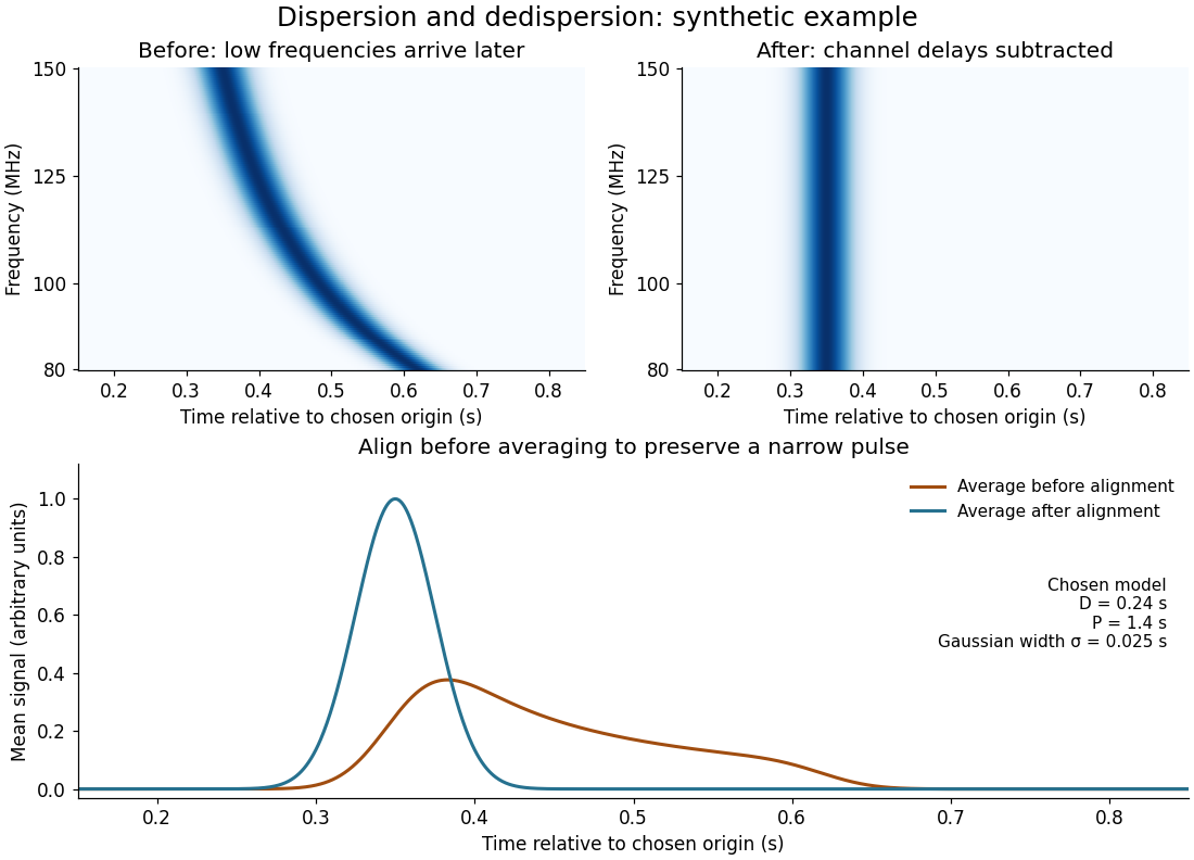
Pulsar dedispersion aligns radio wave arrival times in separate frequency channels before combining them. For an original illustrative model chooseBoth bracketed ratios are dimensionless, so supplies all the time units. The reference is : delays are there, at , and at . These are chosen model values, not measurements of the first pulsar. Subtracting the delay aligns the peaks; summing channels first spreads a short pulse over a longer interval and reduces its peak. Finite channel width and incorrect delay parameters leave residual smearing.

Dispersion measure Created 2026-10-18 Updated 2026-10-20
The integrated electron number density along the line of sight, conventionally quoted in . A dispersion measure is a column, not a unique distance: converting it into distance requires a model of the interstellar medium. A clumpy nearby column and a longer dilute column can give the same pulsar dispersion delay.
Receiver-pessimal stable matching 2026-10-18
For fixed strict preferences, the same output of the Gale-Shapley algorithm gives each receiver its worst partner obtainable in any stable matching, treating unmatched as last. "Worst" is restricted to stable possibilities: a receiver might still receive its favourite acceptable partner if every stable matching assigns it that partner. Reversing the proposing side gives receivers their best stable partners instead.
For a short proof, let be a proposer-optimal stable matching and any other stable matching. If a receiver preferred to , then proposer optimality would make prefer to , since the partners differ and preferences are strict. The pair would block . Therefore no receiver prefers its partner in to its partner in . In the worked example, right-side ranks in are for , whereas gives them . Neither outcome is universally best for both sides.
Change of variables for probability densities Created 2026-10-18 Updated 2026-11-05
For a random variable with probability density function on an interval, let , where is a diffeomorphism onto another interval. The change of variables formula givesIndeed, integrating the right-hand side over an outcome interval gives the probability that lies in its inverse image. The absolute derivative preserves positive probability when reverses orientation. A gravity deflection of an atomic beam is a physical example: its speed-to-height transformation changes the probability density and its mode.
KHP standardization protocol 2026-10-18
Columbia University's institutional laboratory manual, Experiment 1, Glassware Calibration, Primary and Secondary Standards, and Manual Titrations, Part 3, specifies two weighed – portions of potassium hydrogen phthalate, transferred completely into separate Erlenmeyer flasks. Dissolve each in approximately distilled water; any warmed sample cools to room temperature before titration. Add two or three drops of phenolphthalein. Rinse and condition a clamped burette with the diluted sodium hydroxide, then titrate while swirling to faint pink lasting about seconds. Calculate concentration from each portion's own mass and delivered titre; repeat if results scatter. Part 1 identifies a Mettler balance, and Part 2 includes paired weighings of exposed sodium hydroxide and potassium hydrogen phthalate. These are prescribed procedures, not reported measurements.[ref]
The same manual directs keeping the diluted sodium hydroxide covered and limiting air exposure after titrant standardization.[ref]
Glassware Calibration, Primary and Secondary Standards, and Manual Titrations, Columbia University Experiment 1. Experiment 1, Part 3, introductory paragraph and step 1
The MIT handout explains the associated carbon dioxide problem: carbonate contamination of sodium hydroxide is controlled during preparation, bottles are promptly capped, and atmospheric carbon dioxide makes the pink phenolphthalein endpoint fade.[ref]The Potentiometric Titration of an Acid Mixture (MIT 5.310 laboratory handout). Printed Titration-5, §IV.1 and footnote 3; Titration-6, footnote 6
Consequently, a standardized concentration applies to the stored chemical solution under its handling conditions; continued uptake of carbon dioxide can change the reacting inventory per delivered volume.The color is the readout, and stoichiometry supplies the inference. Phenolphthalein indicates a pH range, so its first reproducible pale pink is an operational titration endpoint, rather than a direct observation of equal reacting inventories. A potentiometric titration can locate an endpoint from a pH versus volume curve, but glass electrode calibration alone still does not determine sodium hydroxide concentration. Repeat portions test scatter; incomplete dissolution, an unmatched titration blank, or a shared endpoint error can bias all repeats together.
Primary standard inventory 2026-10-18
Let be the transferred sample mass, the known mass fraction of the intended chemical compound, and its molar mass. In a model with complete dissolution and chemically inactive impurities,The purity fraction is dimensionless: would mean , not . These equations assume that the impurity contributes no titrant demand; an impurity that also reacts needs its own inventory equation. The value of must refer to the same preparation state as , for example the specified dry material. A mass fraction assigned before unaccounted uptake of water cannot simply be used after it.
For an original worked example, stipulate pure potassium hydrogen phthalate, abbreviated KHP, so , a selected mass , and rounded molar mass . The NIST Chemistry WebBook lists formula and molecular weight , consistent with the rounded molar mass used here.[ref]
potassium hydrogen phthalate. NIST Chemistry WebBook, SRD 69, potassium hydrogen phthalate, CAS 877-24-7; Formula and Molecular weight fields
The selected mass, purity assumption and volumes in this example are chosen inputs, not measured results or a claim about a real batch's purity.The acid-bearing anion of potassium hydrogen phthalate loses one proton to hydroxide. The net chemical equation isThus sodium hydroxide has one-to-one stoichiometry with potassium hydrogen phthalate in this neutralization, givingChoose a delivered endpoint titre of and matched titration blank of . ThenThe extra displayed digits show the arithmetic of the stipulated model; they do not establish experimental accuracy. A compact rounded result is .
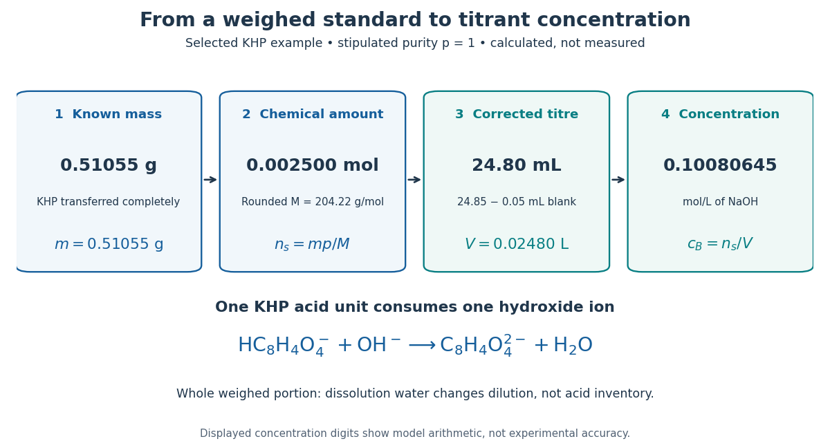
A primary standard connects known mass to amount of substance, corrected titre, and titrant concentration
. Original calculated inventory diagram for selected potassium hydrogen phthalate, stipulated , rounded molar mass , and one-to-one sodium hydroxide neutralization. The endpoint and matched titration blank are chosen examples, not observations. Details.
When the entire weighed portion is titrated, added water changes concentration and the pH path but preserves the initial acid inventory. The dissolution volume therefore does not appear in . If instead a volumetric flask prepares a stock and a volumetric pipette selects an aliquot, the selected inventory is for homogeneous stock, with delivered aliquot volume and final stock volume . The same bookkeeping explains why complete transfer matters even when the amount of dissolution water is approximate.
Resistance pressure gauge 2026-10-18
A resistance pressure gauge is a pressure sensor whose electrical resistance is calibrated against pressure. Even a simple local response needs both pressure and temperature. For an original illustrative model definewhere is the reference electrical resistance at , , and zero history offset. The derivatives and are local sensitivities with units and , respectively; is a dimensionless history offset. Constant sensitivities are an approximation over a chosen range, not material constants valid at every pressure.
Choose synthetic coefficients and , with and . A measured ratio then gives . Ignoring the temperature change gives , a error. This model is deliberately stipulated; these numbers are not measured manganin coefficients or Bridgman's data.
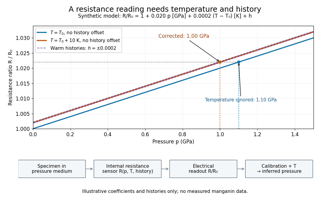
Pressure calibration: a synthetic electrical resistance response with temperature and hysteresis offsets
. Original calculated example. The blue reference line has , ; the orange line has , . Dashed lines illustrate two histories with , not observed data. A ratio 1.022 maps to 1.00 GPa after correcting temperature, or 1.10 GPa if read against the blue line. The lower chain distinguishes the specimen, the internal sensor, the electrical readout and the calibrated pressure. Details.
If two histories differ by , their outputs at the same pressure differ by ; interpreting both with a single history-free curve gives an apparent pressure separation . The half separation is . Reversing the drive can additionally cause mechanical friction hysteresis, independently of this sensor model. Record both the electrical calibration history and the loading direction.
For independent small standard measurement uncertainties and exact stipulated , first-order propagation givesFor , , and , this is . Real calibration also includes coefficient measurement uncertainties, correlations, reference-point measurement uncertainty, and any unresolved nonhydrostatic loading. A sensor calibrates its local environment; it cannot by itself certify the absence of deviatoric stress throughout the sample.
Polar area element Created 2026-10-18 Updated 2026-10-20
For polar coordinates , with , the Jacobian determinant is . The change of variables formula therefore gives the area element . Integrating over the radial interval gives per unit angle. Bounds must describe the intended region without counting it more than once.
Poisson extension of interval boundary data Created 2026-10-18 Updated 2026-10-25
For boundary value on and zero outside, integrating the Poisson kernel for the upper half-plane gives the displayed bounded harmonic function for . It approaches the assigned values at boundary continuity points and the midpoint value at either jump. Changing the value at an isolated endpoint does not alter the integral. This is the unique bounded harmonic extension; pointwise decay in the vertical direction alone, without a spatial growth restriction, does not give uniqueness.
Bridgman unsupported-area seal 2026-10-18
Consider an ideal pressure-driven closure plug with a large chamber-facing projected area . Its opposite side seats against a smaller annular packing surface area . The remaining projected part is the unsupported area: it has no opposing packing contact in that plane. Here is the chamber pressure relative to the exterior. Let denote the mean axial compressive contact stress on the packing, not the chamber's hydrostatic stress.
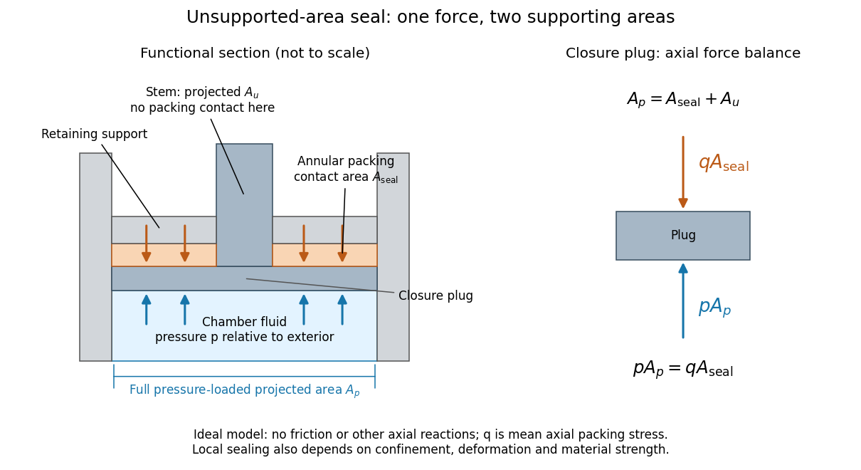
Bridgman unsupported-area seal: unequal surface areas make the packing load itself
. Original functional section and force diagram, with no historical dimensions. Chamber pressure acts over ; the packing reaction acts over the smaller . The central stem occupies the unsupported projected part . Blue arrows show the chamber load on the closure; orange arrows show the opposing packing reaction. The drive piston that pressurizes the chamber is a separate experimental function. Details.
Neglect friction, the plug's weight, and other axial reactions. The plug's Newton's second law in static balance isThe load is the same on both sides; its smaller supporting surface area raises the packing's mean contact stress. For a stipulated ratio and , the ideal seating stress is . Its excess over chamber pressure is . Reducing to zero removes this amplification. This is the elementary force balance behind self-energizing seating, consistent with the lecture's Figure 1 caption.[ref]
The relation is a model, not a universal sealing law. The mean axial contact stress need not equal the local contact stress along every possible leakage path. Confinement and plasticity in continuum mechanics determine whether the packing closes a gap or instead extrudes into it. Friction diverts load into other surfaces; material plasticity in continuum mechanics changes contact geometry; the vessel must carry its own stress. A finite initial seating load may also be needed before chamber pressure can develop. An arbitrarily small does not yield arbitrarily useful sealing: the assumptions fail when local deformation, extrusion or structural failure takes over.
Umklapp scattering Created 2026-10-18 Updated 2026-10-20
An Umklapp process conserves reduced crystal momentum modulo a nonzero reciprocal lattice vector. It can occur in electron-phonon scattering as well as phonon-phonon scattering; the lattice takes up the reciprocal-lattice momentum.
In a three-phonon Umklapp scattering process, the first-zone wavevectors obey the displayed equation for a nonzero reciprocal lattice vector , together with conservation of energy. The crystal momentum transferred to the lattice allows these processes to relax a phonon heat current. They are suppressed at sufficiently low temperature and often determine the approximate high-temperature thermal conductivity of a crystalline electrical insulator.
Phonon mean free path Created 2026-10-18 Updated 2026-11-05
The phonon mean free path is the typical distance traveled by a phonon between the relevant scattering events. For heat transport, the relevant relaxation time must describe relaxation of heat current, not merely count all collisions. An isotropic kinetic estimate is , where is heat capacity per unit volume. Boundary-limited and the low-temperature Debye model give .
Monatomic-chain dispersion relation 2026-10-18
For equal masses at spacing joined by nearest-neighbour springs of spring constant , Newton's second law gives . A normal mode givesThis single acoustic phonon branch is linear at small wavevector and has zero group velocity at the first Brillouin zone edge.
Diatomic-chain dispersion relation with equal springs Created 2026-10-18 Updated 2026-11-05
For alternating masses at spacing , equal nearest-neighbour spring constants , and cell length , a two-component normal mode givesThe minus sign is the acoustic phonon branch and the plus sign is the optical phonon branch. For the edge frequencies are and , leaving a gap. At they are zero and .
Bromothymol blue 2026-10-18
Bromothymol blue is a pH indicator used to assign a color-based titration endpoint in the inspected solubility product measurement by titration.
There are unlisted articles, also show them or only show them.