
For a real conductivity tensor invariant under every rotation about a unit vector , the electric current density is . Its collinearity with a nonzero real electric field has three cases. Axial fields are always mapped to an axial current. Purely transverse fields give a collinear current exactly when , equivalently when this tensor is symmetric. Fields with nonzero axial and transverse parts require both and , making the tensor isotropic. The zero vector is included as a scalar multiple; requiring a nonzero current also requires the relevant scalar conductivity to be nonzero.
For two masses, connect each to a fixed anchor and to the other mass with equal stiffness . Set to choose units. The squared angular frequencies have characteristic equation . Requiring a frequency ratio of two means that these roots are and . Their sum and product give , yielding the two reciprocal ratios in the header. Restoring units multiplies all squared frequencies by , leaving the permitted mass ratios unchanged. The term octave refers here only to this two-to-one ratio.
Elliptically scaled angular one-form 2026-10-18
For real , this differential one-form on the punctured plane is the pullback of a differential form of the nonexact angular one-form under the invertible linear transformation . It is a closed differential form for every such pair. On a region admitting a continuous complex argument, it has the local potential . In a chart with , this can be written .
There is no globally single-valued potential on the whole punctured plane. On the closed path , , , substitution gives , hence its line integral is . This contradicts the zero integral around every closed path required of an exact differential form. Around a positively oriented once-winding path the integral is . The local equation gives radial rays; away from a vertical ray its solutions as graphs are on intervals not crossing the excluded origin.
Node order in Newton interpolation 2026-10-18
Reordering the interpolation nodes changes the successive subsets used for the divided differences and the factors of the Newton polynomial. The final interpolation polynomial remains unchanged in exact arithmetic. For , reversing gives and values . The successive divided difference columns are nowFor example, the first second divided difference is . The top row becomes , givingThe earlier partial interpolants differ because they fit different subsets: fits , whereas fits . The highest divided difference is invariant because both complete top rows finish with the same set of four interpolation nodes; this is symmetry of divided differences.
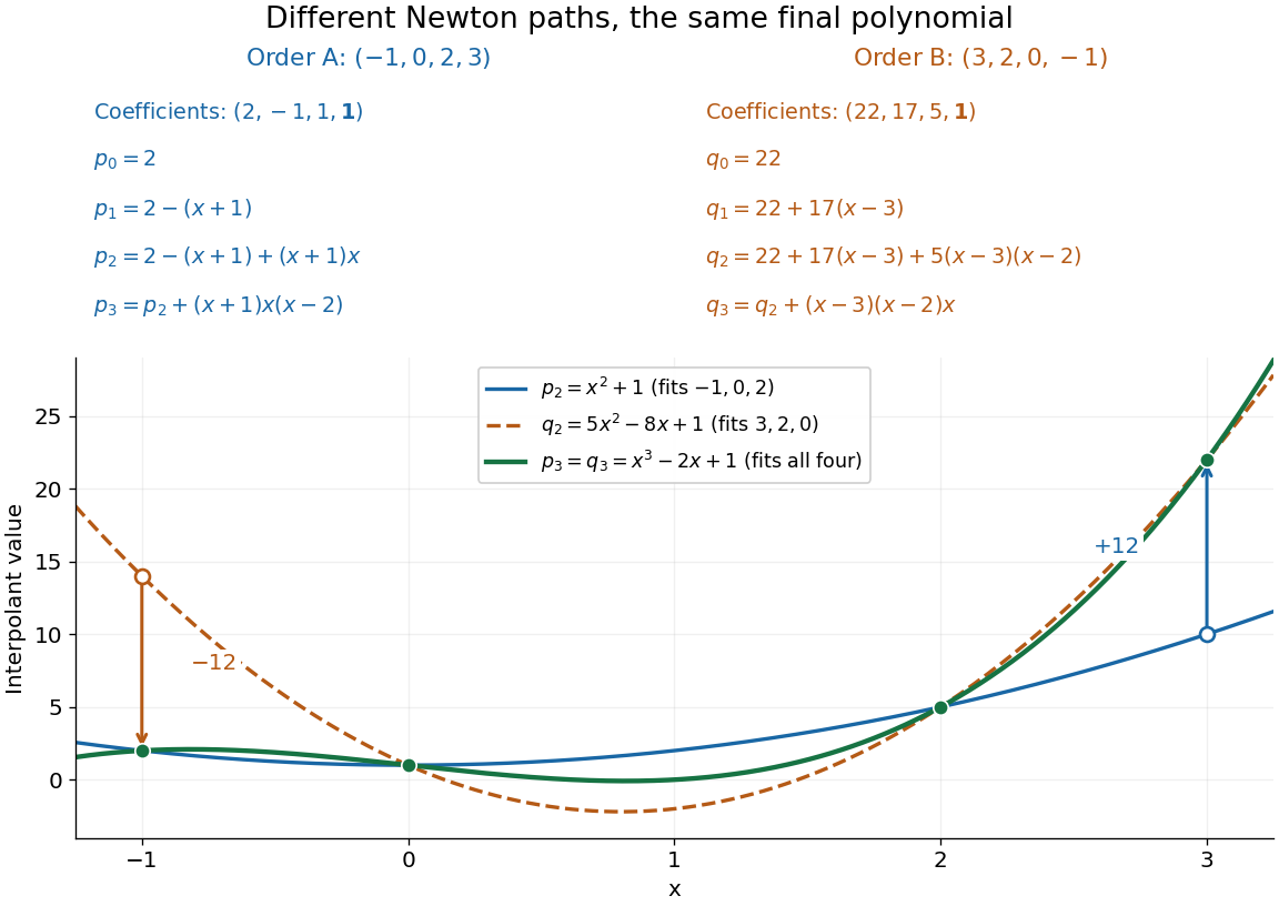
Reversing the interpolation nodes changes the Newton construction but gives the same final polynomial
. Details. 
This distinction is useful when checking a divided difference table: permuting all the interpolation nodes must preserve its final divided difference, even though the intermediate entries change. It also explains why data can be appended in their arrival order. In floating-point arithmetic, the subtractions and divisions may accumulate different rounding errors in different orders; exact invariance describes the mathematical polynomial, rather than guaranteeing bit-for-bit equality of numerical results.
Mean logarithmic energy decrement 2026-10-18
Consider a nonrelativistic particle of mass undergoing an elastic collision with a stationary free target of mass , where . Assume the outgoing direction is uniformly distributed over solid angle in the center of mass frame; this assumption concerns the scattering angle distribution and need not hold for every target or energy. Let be the cosine of that frame's scattering angle. Transforming the outgoing velocity back to the laboratory givesThe uniform distribution of on makes uniform on . For , integration yieldsFor equal masses, take the limit : . The expected value of the fractional energy after a collision is instead . These are different averages: averaging a logarithm does not give the logarithm of an average.
For independent collisions with the same distribution, the logarithms of successive energy ratios add. ThusHere is the geometric-mean energy, and is a characteristic collision count for reaching an energy scale . It is not an exact first-passage expected value. Individual histories fluctuate, and neither the time between collisions nor absorption is specified by this model.
Neutron moderator Created 2026-10-18 Updated 2026-10-20
A material used for neutron moderation, such as water or paraffin wax in the Fermi slow-neutron activation experiment.
Two-atom neutron diffraction selection 2026-10-18
Choose a one-dimensional crystal with cell translation and two atoms per cell at and . Here is an intracell displacement, distinct from the interplanar spacing above. In a single-scattering approximation, a row of cells has scattering amplitudeThe sum selects reciprocal lattice positions as becomes large. At these positions, the two-site crystal basis structure factor and its squared magnitude areConsequently gives even reflections of strength and extinguishes the odd reflections. Choosing , instead gives and : the odd/even ratio is . Equal atomic numbers would not establish equal if the isotopes differ. The figure below plots these chosen coefficients, without assigning them to actual elements. Missing reflections can encode destructive wave interference within a cell, not the absence of matter at a site.
Nuclear neutron scattering length 2026-10-18
The nuclear neutron scattering length is the effective length coefficient for low-energy nuclear scattering amplitude. For the elementary coherent calculation below, use a bound coherent coefficient for each site, and neglect absorption so that is real. This coefficient describes the atomic nucleus, including its isotope and nuclear spin dependence; it is not proportional to atomic number. Replacing nuclear coefficients by electronic magnetic moments would describe a different scattering channel, with additional direction and spatial-distribution factors, as explained in magnetic neutron diffraction.
Variance of nested measurements 2026-10-18
For pots per treatment and leaves per pot, the group sample mean decomposes into two averages:The variance of a sum adds the variances of the independent terms. Every pot random effect has weight , whereas each remaining error has weight , giving the short proofThis is also the variance of the arithmetic mean of the pot sample means, each with variance . Equal numbers of leaves per pot make the two averaging procedures identical.
If all leaf measurements were falsely treated as independent, the predicted variance would instead be . The ratio of correct to false variance isThus pseudoreplication can underestimate a standard error by the square root of this ratio. Equality holds when or ; sharing a pot creates an error here precisely when the shared influence has positive variance.
Choose , , and as constructed model parameters in squared length units. These are assumptions rather than fitted experimental values. For each group,The treatment contrast has expected value . Since the group errors are independent conditional on the allocation, its variance is twice the group variance, namely , whereas the false calculation gives . Its correct standard error is length units; the false value is . The variance ratio is .
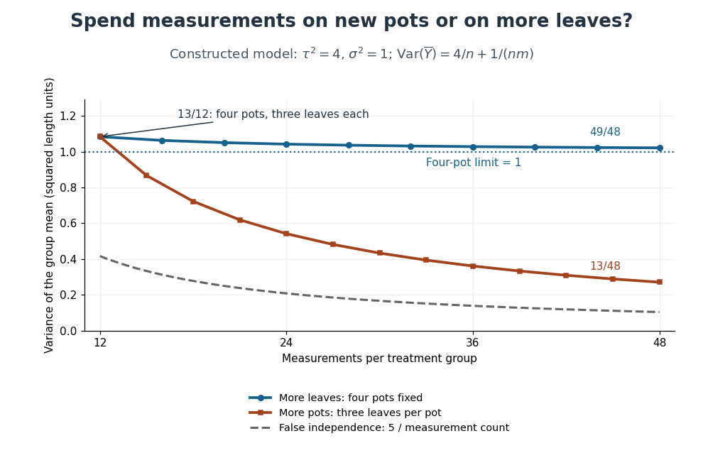
Constructed variance predictions: adding pots reduces uncertainty faster than adding leaf measurements within four pots
. Each curve uses and ; the horizontal axis counts measurements per treatment. The solid designs agree at four pots with three leaves each. The dashed curve assumes all measurements are independent and therefore illustrates pseudoreplication; none of the curves are observed experimental data. Details.
With four pots fixed, increasing drives the error contribution towards zero, but the limit of the group variance remains . Measuring twelve leaves on each of four pots gives . Using the same forty-eight measurements on sixteen pots, with three leaves per pot, gives . More independent experimental units reduce both contributions. Extra nested measurements are useful for characterizing each experimental unit, but cannot average away its shared random effect. This is why sample collection effort and the number of independent treatment replicates answer different questions.[ref]
Pseudoreplication and the Design of Ecological Field Experiments by Stuart H. Hurlbert. Pseudoreplication and the Design of Ecological Field Experiments, p. 201, “Multiple samples per experimental unit”
Suppose independent Bernoulli trials give a player a win with probability , and the match ends when either player reaches wins. The player's match-win probability isFor a win with losses, the final trial must be a win. The preceding trials contain exactly wins and losses; the binomial coefficient counts their arrangements. Because , the opponent cannot already have won, and because the player has only previous wins, the match has not ended earlier. Summing the disjoint terminal events gives the formula, a truncated negative binomial distribution sum. The constant game-win probability must describe independent games, or equivalently remain the same conditional on every previous history.
Success-failure stopping identity Created 2026-10-18 Updated 2026-10-20
In independent Bernoulli trials with success probability and failure probability , let be the trial of success and the trial of failure , for positive integers . If success occurs after failures, its final trial is a success and the preceding trials have successes and failures. The negative binomial stopping argument therefore gives the title sum.
Put . By trial , at least one target must have been reached, so the same event is that a binomial distribution with trials has at least successes. Conditioning instead on the final trial of a block of trials givesIndeed, more than successes in the full block guarantee the success target won; with exactly successes it won only when the final trial was a failure. These disjoint cases explain the extra boundary term. A zero success target wins immediately; a zero failure target has already been reached. To include in the displayed finite sum requires the explicit generalized convention ; an upper summation limit of denotes an empty sum.
The natural logarithm has the parameter-integral representationFor , the identity shows convergence: the absolute value is at most , which is integrable when . At , the apparent singularity is removable, with limiting value .
Write the left side as . On a compact parameter interval with , its differentiated integrand is bounded by the integrable function . The dominated convergence theorem justifies differentiation under the integral sign, giving . Since , the fundamental theorem of calculus gives . At , the original improper integral diverges as , and it also diverges for .
Mercator series 2026-10-18
Integrating the geometric series for from zero to gives the displayed power series for . It has radius of convergence one. At the alternating series test gives conditional convergence to ; at the negative harmonic series diverges. Replacing by gives . An expression formed by substituting a nonlinear function for need not have the same convergence range after it is re-expanded as a Taylor series in the new variable.
Albert Abraham Michelson's 1907 lecture, Recent Advances in Spectroscopy, pp. 171–172, connects counting interference fringes with a reproducible length standard. Broad or multiple spectral lines obscured fringes at large path differences; red cadmium emission supplied a suitable source. His 1907 Nobel Prize in Physics recognized optical precision instruments and their spectroscopy and metrology applications.[ref]
Recent Advances in Spectroscopy by Albert Abraham Michelson. Nobel Lectures, Physics 1901–1921; Michelson, Nobel lecture, printed pp. 171–172; official prize motivation, printed p. 158
His authored account of the metre comparison at Sèvres describes a heated, evacuated cadmium discharge tube and a spectrometer selecting one spectral line. A movable reference mirror was compared with pairs of silvered parallel surfaces defining intermediate standards. Counted interference fringes established a short interval; repeated comparisons extended it to a decimetre and then a metre. White-light fringes located surface coincidence, while monochromatic fringes supplied counts and fractional orders. A thermally shielding box, firm pier, calibrated translation screw and tested thermometers controlled drafts, vibration, travel and temperature. Uniform temperature mattered in comparisons; the final standard required an absolute temperature reading. Optical microscopes made the final comparison to the marked metre bar, limiting the whole result.[ref]
Lecture V: Light Waves as Standards of Length. Michelson, Light Waves and Their Uses (1903), Lecture V, Figs. 70–77: intermediate standards, counting, temperature controls and final microscope comparison
This is a measurement chain, rather than one enormous unchecked fringe count: short intervals establish whole orders; fractional-order readings refine each longer comparison. The optical coherence envelope helps locate white-light coincidence, whereas the carrier phase difference measures small departures from it. Repetition checks counting mistakes, but agreement alone cannot exclude shared systematic errors. The general lesson of metrology is to preserve the link from the optical ruler through each transfer and control to the final length.
Precision displacement measurement with a Michelson interferometer Created 2026-10-18 Updated 2026-10-20
A Michelson interferometer turns displacement into a count of interference fringes: a moving mirror changes both the outward and return paths. This lets a wavelength act as a ruler whose divisions need no engraving. Assume normal incidence, a fixed reference arm, stable refractive index along the moving arm, and fixed vacuum wavelength . Write for the wavelength in that medium and take positive away from the beam splitter. The change in optical path difference, the accumulated phase difference, and the signed number of complete interference fringe cycles areThe factor two comes from propagation geometry: moving the mirror by adds before reflection and afterward. One bright-to-bright cycle means mirror travel ; bright-to-dark means , half a cycle. All lengths must use compatible units, and is dimensionless. A constant reflection phase difference changes the initial fringe position but cancels from this change formula.
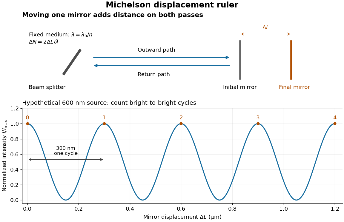
Mirror displacement, doubled optical path difference, and counted interference fringes for a hypothetical Michelson interferometer
. Details. 
For an original hypothetical example, suppose in the actual surrounding medium and a continuous scan gives cycles, including the final fractional cycle. Then . With the wavelength treated as exact, a fringe-reading measurement uncertainty of cycle contributes to the displacement measurement uncertainty. An uncertainty of in a local phase difference instead corresponds to . This illustrates measurement resolution, not a complete claim of accuracy: wavelength calibration, air changes, mirror tilt and missed cycles can dominate.
To separate the oscillating readout from its optical coherence envelope, use the local modelHere is detected light intensity, is the mean level, is a fixed bias wave phase, and is interferometric visibility. A fine scan of measures the carrier phase difference; a coarse scan can map the temporal optical coherence envelope through . The envelope maximum locates matched delays only under the source and apparatus assumptions; it is not a bright fringe identifying an arbitrary mirror position. Even with known , one intensity reading leaves the cosine sign and whole-cycle ambiguities. Continuous motion of known direction, or an independently obtained pair of signals in phase quadrature, is needed to recover signed travel through reversals.
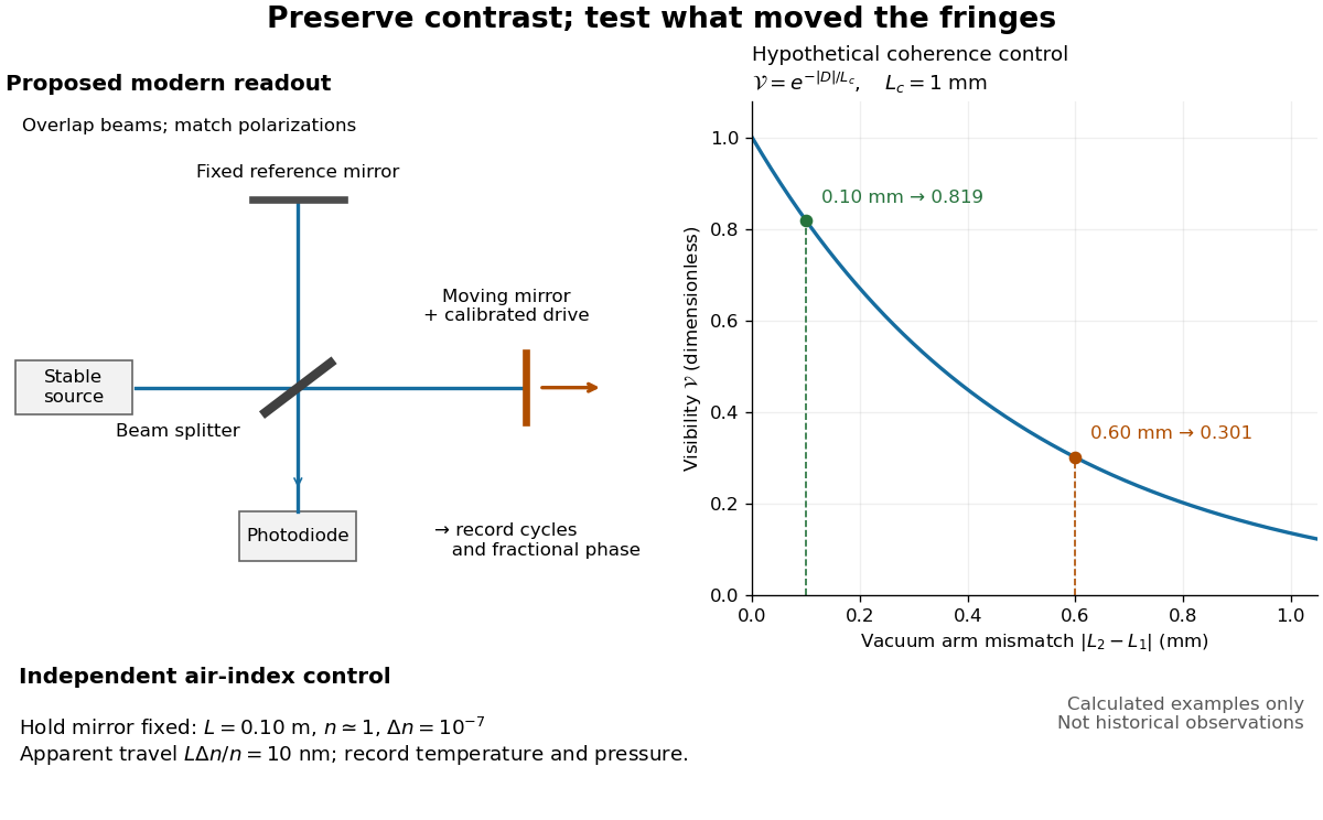
Proposed Michelson interferometer readout and hypothetical optical coherence and refractive index controls
. Details. 
The figure's original control example stipulates equal arm light intensities, matching linear polarizations, and a Lorentzian optical spectrum giving with . In vacuum, arm mismatches and give and . Matching the arms improves the phase difference readout without changing its travel per cycle. A fine mirror scan of one cycle changes by only for the stipulated source, much less than . These are calculated values, not historical data.
A proposed measurement sequence follows from this model. Overlap the returning beams, match their linear polarizations, find a high-contrast delay and use a small calibrated mirror scan to determine the sign and fringe period. Read a fixed spatial sample of the interference fringes with a photodiode; record each arm separately and the dark signal, avoid detector saturation, and retain enough time resolution to count every cycle. Approach mechanical settings consistently and repeat the return scan to expose lost motion or drift. For very small changes, bias near phase quadrature, where is largest; an intensity extremum has zero first-order sensitivity. A known drive voltage alone does not provide measurement calibration for mirror travel: compare the actual travel with the fringe count using an independently known wavelength.
Control temperature, pressure, vibration and air currents because the instrument measures optical path difference, not mirror motion alone. For a fixed reference arm and fixed , the first-order change of the moving arm's round-trip path is . Thus an unrecognized mimics . A hypothetical , , and give apparent travel. Holding the mirror still while varying or monitoring the air conditions tests this confounder. Separate checks of alignment, wavelength stability and thermal expansion are necessary before sub-fringe measurement resolution becomes a defensible measurement uncertainty.
Matrix powers for a diagonalizable matrix with two eigenvalues Created 2026-10-18 Updated 2026-11-05
If a diagonalizable matrix has distinct eigenvalues , its spectral projections of a diagonalizable matrix are and . Raising the diagonal form to a nonnegative integer power gives the displayed formula. Equivalently, interpolate the scalar function by a degree-one polynomial at , then apply it to . The diagonalizability assumption matters: knowledge of two eigenvalues alone does not exclude nontrivial Jordan blocks.
Diagonal matrix entry Created 2026-10-18 Updated 2026-10-25
A diagonal matrix entry uses the same row and column index. The diagonal entries of a lower triangular matrix determine its determinant by their product.
Spin valve 2026-10-18
A device with a reference magnetic layer whose magnetization is comparatively fixed and another layer whose magnetization responds more readily to an applied field. The resistance reads their relative alignment. Fert's account describes how such giant magnetoresistance sensors entered hard-disk read heads in 1997.[ref]
Nobel Lecture: Origin, development, and future of spintronics by Albert Fert. p.1519, spin-valve structure and historical read-head adoption
Giant magnetoresistance 2026-10-18
Giant magnetoresistance connects the relative magnetizations of adjacent magnetic layers to their electrical transport. In a suitable magnetic-metal/nonmagnetic-metal stack, aligning the layers can leave one spin channel with an easy conducting path through both magnetic layers; opposite alignments make each channel encounter a more resistive layer. Albert Fert's account traces the spin-dependent-conduction idea to Nevill Mott and distinguishes the later device geometries.[ref]
Nobel Lecture: Origin, development, and future of spintronics by Albert Fert. pp.1517–1520, spin-dependent conduction and CIP/CPP geometry
The beauty is that a magnetic arrangement becomes an electrical readout. Preparing reproducible layers, establishing their magnetizations, and measuring electrical resistance are separate parts of that inference. The Fe-Cr giant magnetoresistance experiments show how those parts were joined; the two-current resistor model isolates a simple transport mechanism under stated assumptions.
There are unlisted articles, also show them or only show them.