
Finite-scale vortex renormalization 2026-10-18
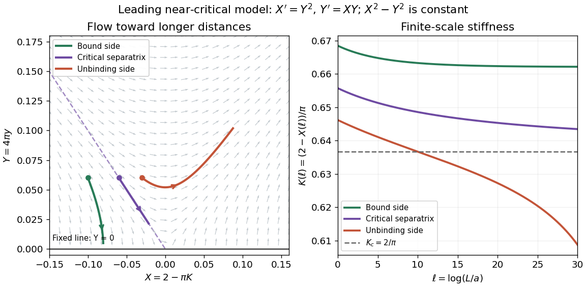
An experiment of size stops the renormalization-group flow at a finite . In the leading scaled model take the original initial conditions and . The invariant is respectively . The first approaches , hence ; the second follows the critical separatrix; the third eventually leaves the small-vortex fugacity regime. These are chosen model trajectories, with no fitted experimental parameters.
On the critical separatrix, implies , henceEven a critical finite sample therefore has a phase stiffness above its asymptotic jump value, with a slow logarithmic correction in . Slightly above the transition, a sample with can resemble the algebraic phase before the flow reaches unbound vortices. A trap additionally varies the local density and phase stiffness; neither its whole-cloud coherence nor a finite observation window automatically measures the homogeneous thermodynamic limit.

Vortex fugacity 2026-10-18
A dimensionless statistical weight per microscopic phase vortex core. In a dilute convention it is , with core energy and a specified microscopic integration measure. Its numerical normalization fixes coefficients in the vortex-pair renormalization flow.
Volume of a solid with affine thickness 2026-10-18
Let a bounded planar region have positive area and centroid . If a solid has nonnegative thickness above , its volume integral givesThus the average of an affine function over a region is its value at the centroid. The proof is the linearity of integration. For a disk the centroid is its centre, making the formula particularly useful for a cylindrical bore cut through a solid whose width varies linearly with height.
Euclidean scalar-gradient stress identity Created 2026-10-18 Updated 2026-10-25
For a sufficiently smooth real scalar field on Euclidean space, set . The product rule and equality of mixed partial derivatives giveThe divergence theorem, applied twice, consequently gives the useful pure-boundary identityHere uses the outward unit normal. This is the Euclidean zero-potential counterpart of the scalar stress-energy divergence identity.
Van der Waals molar equation 2026-10-18
The molar volume is the volume per amount of substance, not the total container volume or the volume per particle. In the molar convention of the Van der Waals equation, take constant positive parametersThenor, for any fixed amount of substance,Both terms in the first equation are pressures. The total excluded volume is : using would subtract quantities with different units. Changing the sample size at fixed molar volume and temperature changes and proportionally, while leaving pressure unchanged. This is a useful unit and extensivity check before fitting a real gas.
For the molar Van der Waals critical point, differentiate with respect to molar volume at fixed temperature:Setting both to zero gives and . Equating them and dividing by the nonzero factors yields , soHere has units , has units , and has units . This is the molar version of the particle derivation below: , with the same physical and . If one writes , and without subscripts, then all of in those formulas must be molar quantities.
Now define the dimensionless reduced variables explicitly as , and . Substituting the three critical values cancels and givesBecause , these are exactly the reduced variables in the Van der Waals isotherm discussion. The Van der Waals law of corresponding states is therefore independent of whether one starts with particle or molar units. It predicts a critical ratio , providing a third check on any proposed parameter fit.
Entropy excess of a van der Waals gas Created 2026-10-18 Updated 2026-11-05
For one mole with temperature-independent parameters , the equation of state is . A Maxwell relation gives , so the volume dependence is . Matching the ideal gas entropy at infinite volume fixes the excess at the same to . The attraction contributes to the Helmholtz free energy but no excess entropy when is independent of temperature. A temperature-dependent attraction parameter would change this conclusion.
Internal energy of a van der Waals gas Created 2026-10-18 Updated 2026-10-20
For fixed amount of substance, thermodynamic consistency givesIndeed, the first law of thermodynamics gives , and the Helmholtz free energy Maxwell relation gives . For the fixed-amount convention with temperature-independent , substitution gives . Integration yields . If the dilute-limit reference is as for every , then .
The same formula may be interpreted molarly if all use that convention. Mixing molar and total quantities changes the amount factors. The attraction controls the volume correction to internal energy, while excluded volume alone does not contribute to this derivative when are independent of temperature.
For with , put . The initial conditions and giveThus the turning points have the times and displacements in the title. For release from , the first positive maximum is , sufficient to test whether the body reaches a fixed positive stop before that first maximum. Every later positive maximum is smaller.
Thermomechanical effect 2026-10-18
The thermomechanical effect couples a temperature difference to a pressure difference across a superleak. For the closed-chamber model in the apparatus figure, consider neighboring equilibrium states with small velocities, negligible height difference and pure helium-4. Let be chemical potential per unit mass, in . The Gibbs free energy differential per unit mass givesThe superleak allows the superfluid to redistribute until the two sides have equal . Setting therefore givesThe sign matters: heating one side at initially equal pressure lowers its ; inflow raises its pressure until chemical balance is restored. The hotter side has the higher pressure. The integral follows the constant- path; it need not be evaluated at fixed pressure when material properties vary appreciably.
For an original local example, stipulate constant , and . The predicted pressure difference is . These are teaching assumptions, not helium measurements. This static thermodynamics relation predicts neither the required heater power nor the filling time: those require heat leakage, channel conductance and chamber heat capacity. An outlet would introduce kinetic energy and a flowing balance, so the static is not a predicted fountain height.
Second sound Created 2026-10-18 Updated 2026-10-20
Second sound is an entropy and temperature wave. At negligible thermal expansion, it has almost zero net mass flux. Lev Davidovich Landau predicted two sound modes in 1941.[ref]
The Theory of Superfluidity of Helium II by Lev Davidovich Landau. Landau, §8, pp.515–516
Fixed-end spring-chain determinant and its repeated-root limit Created 2026-10-18 Updated 2026-11-05
For equal masses joined to fixed walls by equal springs, the stiffness matrix has diagonal and adjacent entries . Its characteristic determinant obeys , , , . If and , then for distinct roots. At a repeated root , the correct limit is , which is nonzero. Thus the apparent ratio solution must be excluded. Writing gives , the Chebyshev polynomial of the second kind. There are exactly distinct positive normal frequencies , .
If are independent random variables, each with the uniform distribution on for , then has the symmetric triangular distributionThe convolution of probability densities gives . The overlap of these two intervals has length for and is empty otherwise, proving the formula. By linearity of expectation and the variance of a sum,For , its upper-tail probability is .
A useful model for elapsed time measured from two independently truncated clock readings uses as the display resolution and as the endpoint-offset difference. Independence is essential: uniform marginal probability distributions alone do not imply this triangular distribution. For example gives with certainty. In general, with the same uniform marginals, .
Transmission electron microscopy specimen dose and calibration Created 2026-10-18 Updated 2026-10-20
JEOL's minimum-dose method focuses and corrects astigmatism away from the recording position before exposing it, reducing irradiation of the chosen field.[ref] A downstream objective aperture cannot undo irradiation that has already reached the specimen: rejecting more outgoing electrons does not itself reduce specimen exposure.
For an original dose budget, define as incident electron count per specimen area, rather than absorbed energy per mass. A uniform beam of electric current magnitude , illuminating area for time , giveswhere is the elementary charge. Choosing , and gives approximately incident electrons, or . This is an invented exposure calculation, not a safe-dose recommendation. Focusing and searching exposures must also enter the accumulated budget.
If detected counts follow a Poisson distribution, a mean count has standard deviation . Ignoring background, accepted counts therefore have relative counting uncertainty, while have . Reducing accepted counts can reveal useful diffraction contrast while increasing counting uncertainty. It is useful to specify both contrast and count budget when discussing electron microscope resolution.
A proposed measurement calibration sequence records a beam-blocked detector background, an illuminated empty support region, and a specimen image with fixed voltage, exposure and detector gain. Test detector linearity with exposure time before comparing corrected intensities. Calibrate the image scale against a known spacing, as in microscope scale calibration, and independently calibrate electron diffraction spacing at its own lens settings; one calibration does not supply the other. Register compared regions, record objective aperture selection, specimen tilt and accumulated exposure, then repeat the first setting to test drift and irradiation changes. These are proposed controls, not undocumented steps attributed to JEOL's silicon example.
Transmission electron microscopy contrast Created 2026-10-18 Updated 2026-10-20
Transmission electron microscopy contrast is a difference in recorded signal between specimen regions under specified illumination, angular acceptance and detector settings. For a positive reference signal , one possible signed contrast convention isNegative means darker than the reference; it does not specify a surface height or chemical composition. The definition must accompany a numerical contrast value, since other conventions exist. A conspicuous feature need not establish fine spatial resolution: detecting a small signal difference and distinguishing two nearby features are different measurement questions.
Top-quark decay before hadronization Created 2026-10-18 Updated 2026-11-05
Here , and the tree-level decay width neglects the bottom quark mass. The open two-body W channel gives a top quark lifetime of a few , shorter than the hadronization time. A fifth-power Sargent's rule extrapolation misses this physical regime.[ref]
Review of Particle Physics by Particle Data Group (2022). Top Quark review, section 61.2, equation 61.1 and the accompanying lifetime discussion
pH indicator 2026-10-18
A pH indicator changes color as its protonation distribution changes. In a simple weak acid/conjugate base model, its two forms have different colors and their ratio depends on pH through the acid dissociation constant. The visible transition spans a range of pH; it is not a direct signal that the sample has reached an equivalence point. An indicator is useful when its transition lies in a steep part of the titration curve, so a modest range of pH corresponds to a small added volume.[ref]
14.7 Acid-Base Titrations. Chemistry 2e, §14.7, Acid-Base Indicators, Figures 14.19–14.21: indicator equilibrium, transition ranges, and selection
Potentiometric titration 2026-10-18
A potentiometric titration monitors an electrode electric potential difference as titrant is added. A calibrated glass electrode can report pH during an acid-base titration.
Standardization endpoint and blank bias 2026-10-18
Hold the known primary standard inventory fixed, and let be the correct blank-subtracted titre. In the following model, any remaining endpoint offset has been removed from this reference. If a titration endpoint overshoot adds , the inferred titrant concentration is too small:The denominator grows while the numerator stays fixed. For , the relative effect is approximately , but the displayed fraction is exact for this additive model. An unremoved positive titration blank has the same mathematical effect: replace by . If both remain, replace it by . This analogy concerns their effects on the denominator; it does not mean a blank measures endpoint overshoot.
For the chosen reference titre, an extra gives and relative error . Leaving both a blank and a overshoot gives denominator and relative error .
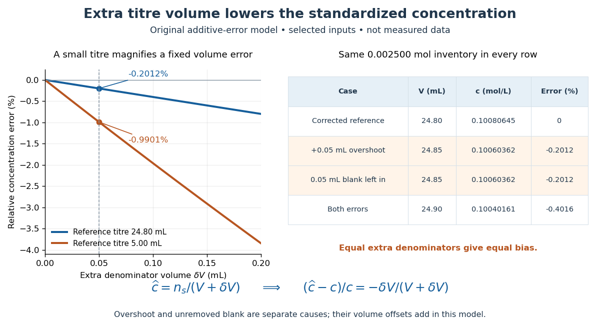
Endpoint overshoot and an unremoved positive titration blank both lower the inferred titrant concentration
. Original additive-error model, not measured data. The curves compare reference titres of and . The table uses the selected inventory and reference. Equal extra denominator volumes give equal bias, whether caused by overshoot or an unremoved blank. Details.
For comparison, the same extra on a reference titre gives . The ratio of these error magnitudes is , while the small-error approximation would give . A larger titre reduces the fractional effect of a fixed extra volume; it does not fix unknown purity, incomplete transfer, or an incorrect stoichiometry.
Titration blank 2026-10-18
A titration blank runs the background procedure without the intended reacting sample, matching relevant water, indicator quantity and titration endpoint conditions. Its titrant demand estimates a background contribution to subtract. The inspected EPA procedure uses such a phenolphthalein blank; this is a distinct control, rather than an instruction present in Columbia's Part 3.[ref]
Process Measurement Procedures: Sulfuric Acid Emissions by R. Maddalone and N. Garner. Printed pp. 26–27, §1.4.4.2, indicator-blank paragraph and steps 1–3: water replaces acid, indicator quantity matches, blank volume is subtracted
A blank must match the relevant background to justify subtraction; it does not remove sample-specific side reactions or a mismatch between titration endpoint and equivalence point. Titre 2026-10-18
Here a titre means the delivered titrant volume needed to reach the specified titration endpoint, obtained from final minus initial burette readings. Report explicitly whether a quoted titre includes or excludes a titration blank. This volume convention is distinct from uses of titre to express a solution's reacting strength.
There are unlisted articles, also show them or only show them.