
Image charges for a neutral conducting sphere Created 2026-10-18 Updated 2026-10-20
A real charge at outside a spherical conductor of radius has the usual grounded-sphere image charge at . Adding a central image makes the total image charge zero, representing an isolated neutral conductor. The off-centre pair has zero potential on ; the central image therefore sets the constant conductor potential to . Its induced electric dipole moment is . Keeping the applied central field fixed gives . As , the external field becomes uniform near the sphere; its divergent constant potential can be removed without affecting the electric field.
Inverting operational amplifier Created 2026-10-18 Updated 2026-11-05
Connect a resistor from the input source to the inverting input, a feedback resistor from output to that same input, and ground the non-inverting input. For ideal linear operation the inverting node is a virtual ground. Kirchhoff's current law gives , yielding the displayed voltage gain. The source sees input impedance , even though the amplifier input itself has infinite input impedance.
Diamond anvil cell 2026-10-18
A diamond anvil cell compresses a sample between opposed diamond tips. The flat diamond anvil culets load a metal gasket whose hole holds the specimen and a pressure-transmitting medium. Transparent diamond admits excitation and returning fluorescence, enabling an internal ruby pressure sensor.[ref]
High Pressure X-Ray Crystallography With the Diamond Cell at NIST⁄NBS by Gasper J. Piermarini. Sections 2–3, Figures 1 and 5: anvils, optical path and gasket
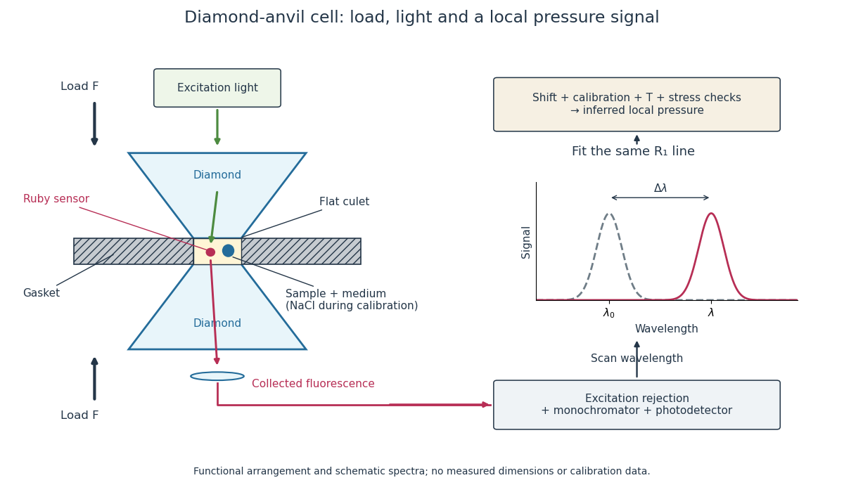
Diamond anvil cell: compression, optical access and internal ruby readout
. Original functional section, not a reconstruction or a scale drawing. The separate excitation and collection paths depict one possible arrangement. A monochromator and photodetector resolve the fluorescence emission spectrum; the inference uses a spectral line position rather than its brightness. The optional sodium chloride reference belongs to the calibration experiment, rather than to every subsequent sample measurement. Details.
The functions in the drawing answer different questions. The drive applies force, the gasket confines the sample, the medium transmits stress, and the ruby pressure scale assigns a local pressure from an optical signal. A large drive reading cannot establish either the sample's pressure or the absence of deviatoric stress. Optical access also permits repeated readings without unloading the sample: a change during a long measurement can be detected rather than silently folded into a material-property curve.
Pressure calibration 2026-10-18
Pressure calibration assigns pressure values to a sensor's output by comparison with a reference under specified conditions. It is not the same as making the output more finely resolved. A smooth electrical resistance curve can be repeatable yet have an incorrect pressure scale.
Bridgman used pressure-dependent electrical resistance of manganin and established fixed points, including a bismuth transition. He reported poorer accuracy above the better calibrated range.[ref]
General Survey of Certain Results in the Field of High-Pressure Physics by Percy Williams Bridgman. p. 56, pressure-measurement paragraph: manganin gauge, bismuth fixed point, and different accuracy estimates below and above 30000 kg/cm²
A fixed-point specimen and a property-measurement sample have distinct roles: one helps assign the scale, while the other is studied on that scale. The reference transition must itself have an assigned pressure at the relevant temperature. Agreement at a single point does not determine a nonlinear sensor response elsewhere. Comparing increasing and decreasing pressure checks hysteresis; returning to a reference checks drift. These are checks one can design from the measurement model, not additional historical controls asserted for the lecture's experiments.
Hydrostatic stress 2026-10-18
With tension taken positive, hydrostatic stress is the stress tensor , where is the identity matrix. Every plane has the same compressive normal stress, and no tangential traction. More generally,where is deviatoric stress. Two samples can share the same mean pressure while experiencing different deviatoric stresses. A stationary liquid cannot sustain equilibrium shear stress; a solid transmitting medium can support it. Consequently, a load divided by surface area does not by itself establish hydrostatic sample conditions. A transmitting medium's state at the actual pressure and temperature, and contact between sample and walls, matter.
Bridgman's Figure 4 compares mild steel fractured in tension at atmospheric pressure with steel stretched further in a liquid at .[ref]
General Survey of Certain Results in the Field of High-Pressure Physics by Percy Williams Bridgman. p. 56, Figure 4 caption: atmospheric-pressure tensile fracture versus greater reduction of area in pressurized liquid; historical kg/cm² rendered explicitly as force per area
The imposed tension remains a directional load: the experiment combines confinement with deformation, rather than measuring a hydrostatic stress alone. Its comparison motivates recording the loading path and the surrounding medium as well as pressure; it does not establish a universal fracture threshold for all steels. Piston-cylinder pressure apparatus 2026-10-18
In a functional model, a driven piston reduces the chamber's volume. A surrounding cylinder carries the wall stress; a deformable packing or gasket closes a potential leak path around a moving or removable closure. A sample and a separate pressure sensor occupy the chamber. A transmitting liquid can load the sample on all sides; the sensor's signal passes to an external readout. This is a division of experimental functions, not a scale reconstruction of one historical machine.
For a slowly moving frictionless drive piston of effective surface area , external pressure and inward applied force , Newton's second law at mechanical balance givesThus on a stipulated effective surface area corresponds ideally to of differential pressure. These are illustrative numbers, not apparatus specifications. The effective surface area is the one associated with the pressure difference, not necessarily an external ram's visible cross section. With resisting friction during inward motion, the balance becomes . During outward motion the sign of the friction contribution reverses. An applied-load reading can therefore show hysteresis even when the chamber's actual pressure is well defined.
A resistance pressure gauge instead supplies an internal signal. In a generic electrical readout, measure an electric potential difference with a known electric current and use Ohm's law to infer electrical resistance . This describes a possible readout principle; the lecture passage cited below identifies the sensor material and calibration landmarks without specifying this wiring.
Higgs degree-of-freedom count 2026-10-18
In four spacetime dimensions a massless vector has two physical polarizations, while a Proca field has three. Before rearrangement, the electroweak sector has four vector fields and four real Higgs doublet components, hence twelve propagating degrees of freedom. In the broken description, W bosons of both charges and the Z boson contribute nine, the photon contributes two, and the radial Higgs boson contributes one. The three angular scalar components supply the three additional longitudinal polarizations. Gauge components and constraint variables are excluded from both counts. The gluon sector is unaffected.
Higgs mechanism history Created 2026-10-18 Updated 2026-10-20
In their 1964 paper, François Englert and Robert Brout showed that gauge bosons associated with generators that rotate the chosen vacuum acquire masses while gauge invariance is maintained. Their discussion included both scalar and fermionic models.[ref]
Broken Symmetry and the Mass of Gauge Vector Mesons by François Englert and Robert Brout. pp. 321–323, especially Eq. (6)
Independently, Peter Higgs exhibited a massive vector and a surviving massive scalar field by linearizing a simple gauge theory. His paper explicitly distinguishes this classical calculation from a proof for the full quantized theory. These 1964 mechanisms supplied an ingredient for the later electroweak interaction, rather than the complete Standard Model.[ref]
Broken Symmetries and the Masses of Gauge Bosons by Peter Higgs. p. 508, Eqs. (2b)–(4); p. 509, note 4
Higgs boson discovery in 2012 Created 2026-10-18 Updated 2026-10-20
The ATLAS experiment and CMS experiment searched proton-proton collisions at the Large Hadron Collider at collision energies of and . The ATLAS experiment used silicon tracking, a solenoid, liquid-argon electromagnetic calorimeters and an external muon spectrometer. Its July 2012 paper reported a combined local statistical significance of standard deviations near ; this paper result is distinct from the initial 4 July announcement.[ref]
The CMS experiment used silicon tracking in a solenoid, lead-tungstate electromagnetic calorimeters and external muon chambers. Electrons combine tracks and particle showers; muons combine tracking and chamber hits; photons supply shower energies and directions. Selected and candidates, with , yielded invariant mass peaks. It checked lepton efficiencies with Z boson decays, estimated fake-lepton backgrounds from control samples with relaxed identification, and fitted the smooth diphoton background from data. Its combined local statistical significance was standard deviations near .[ref]
The ATLAS experiment compared signal-plus-background and background-only hypotheses with a profile likelihood, accounting for systematic uncertainties and correlations between decay channels. Diphoton and four-lepton candidates gave precise invariant masses; decays supplied additional evidence with poorer mass reconstruction because of escaping neutrinos. A local p-value concerns one specified mass; scanning masses requires a look-elsewhere effect correction.[ref]
Two-photon decay excludes spin one under the usual assumptions, but does not prove spin zero. A mass peak does not determine every Higgs boson coupling. Production rates, branching fractions and angular correlations require additional tests.[ref]
Electron Yukawa suppression of Higgs production Created 2026-10-18 Updated 2026-10-20
With the conventional electroweak vacuum value , the electron Yukawa coupling is and the physical Higgs-electron vertex coefficient is . Direct s-channel Higgs production in electron-positron annihilation is consequently very small away from a compensating resonance enhancement. This suppression belongs to the coupling at the initial vertex, not to a prohibition on the Higgs boson coupling to W bosons.
Liquefaction enthalpy budget 2026-10-18
Consider an original model of a cold section enclosing a throttle and collecting region, with the precooling heat exchanger outside its boundary. The inlet has mass flow rate and specific enthalpy . The outlets are equilibrium liquid and vapor at one fixed pressure, with specific enthalpies and . Let be the outlet liquid mass fraction, and let be incoming unwanted heat per unit incoming mass. Assume steady flow, no shaft work, and negligible bulk kinetic energy and gravitational potential energy changes. The steady-flow energy balance givesHere is the latent heat per unit mass at the chosen outlet pressure. The mass flow rates of the outlets are and . The formula describes a flowing cold section; a filling vessel with appreciable energy or mass accumulation requires storage terms.
For a deliberately dimensionless example, choosePer unit incoming mass, one quarter leaves as liquid and three quarters as vapor. With zero incoming heat, the same inlet would give . Increasing to reduces to , and reaches the no-liquid boundary. These are chosen model values, not helium property data or a historical yield. In normalized enthalpy units with and , conservation checks directly: .
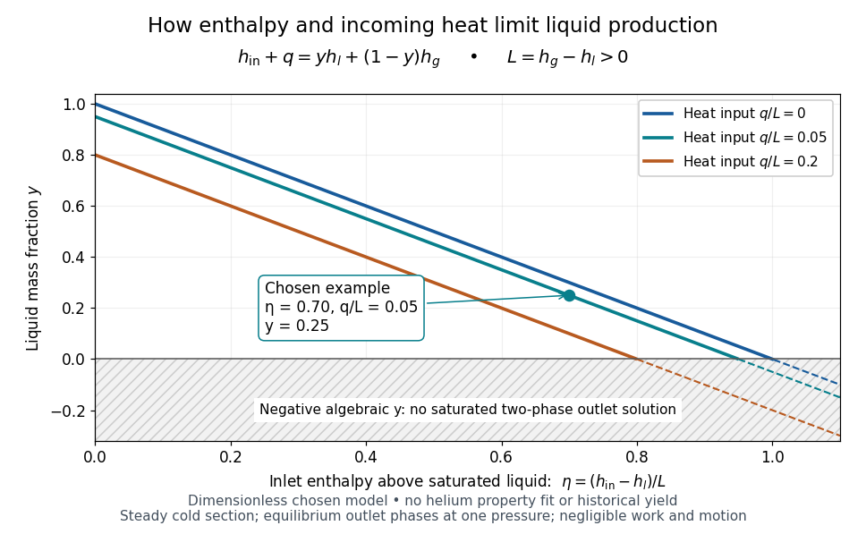
An original normalized liquefaction enthalpy budget
. Each solid segment satisfies the stipulated equilibrium two-outlet model. Dashed negative continuations are algebra only: they do not describe a negative liquid mass fraction. No helium properties or experimental measurements were fitted. Source. Details.
The admissible interval is , or . Outside it, the assumed equilibrium two-phase outlet fails: an enthalpy above requires a hotter single-vapor outlet under these assumptions, rather than a negative amount of liquid. Below , a colder liquid or a different thermodynamic phase must be considered. The balance does not predict its own outlet pressure, temperature or helium property functions.
At fixed outlet pressure, hence fixed , the derivatives are and . Lowering inlet specific enthalpy by regeneration and reducing incoming heat therefore buy the same increase in liquid mass fraction per unit energy per unit mass in this model. Adding any constant to all three specific enthalpies leaves unchanged. This independence of the arbitrary enthalpy reference makes the balance useful even when property tables choose different zero points.
On 10 July 1908, Heike Kamerlingh Onnes's Leiden laboratory circulated purified helium through liquid air and evaporatively cooled liquid-hydrogen precooling, a regenerative heat exchanger, and an expansion valve. Returning helium cooled incoming helium; liquid collected in a transparent vacuum vessel. Reflected light revealed its liquid meniscus, crossed by thermocouple wires. Subsequent mass density and spectroscopy checks tested contamination.[ref]
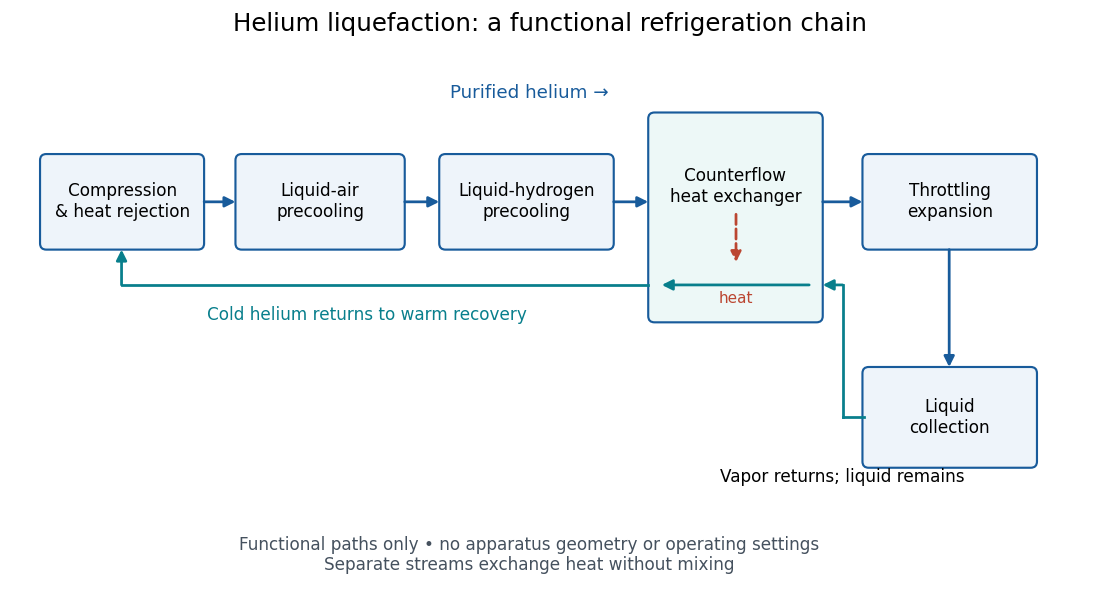
Functional stages of helium liquefaction
. Original functional diagram of the reported sequence. Arrows show stream direction and heat transfer; positions do not represent the apparatus geometry. Compression and heat rejection close the refrigeration cycle. Source. Details.
A constant-volume helium gas thermometer below the valve supplied the temperature indication. An oxygen boiling reference check disagreed with its expected reading; the real gas correction to thermodynamic temperature remained provisional. A temperature plateau suggested immersion before the liquid meniscus was recognized.[ref]
The Liquefaction of Helium by Heike Kamerlingh Onnes. §4, pp. 180–181; §§5–6, pp. 183–184
The measurement principles separate two questions. A visible liquid meniscus establishes an interface; a gas thermometer estimates temperature through an equation of state. A stationary temperature trace can also result from a steady state without phase coexistence, so it cannot replace the interface observation. Conversely, seeing a liquid does not calibrate a thermometer. Thermometer calibration, the gas thermometer dead-space correction, departures from the ideal gas law and incomplete thermal equilibrium all matter when assigning an absolute temperature. A check far from the intended measurement range tests the instrument but does not by itself bound every low-temperature error.
Helium-3 B phase 2026-10-18
Take a proper rotation matrix with real number entries. Then hasThis odd linear orbital model has an isotropic gap magnitude. Isotropic gap magnitude does not require s-wave pairing: the spin components can rotate together with the orbital direction. Nor does the magnitude fix the relative spin-orbit orientation represented by .
For both displayed models, . The triplet gap matrix , written with Pauli matrices, satisfiesThus these models give the same gap magnitude for the two spin branches. That last simplification would fail for a general complex triplet vector with a nonzero cross product. The displayed angular curves illustrate these specified matrices; they are not a microscopic derivation of the phase diagram.
Helium-3 A phase 2026-10-18
Take a real unit vector in spin space and choose orthogonal orbital axes. The model hasIt vanishes at the two polar directions and is largest at the equator. The orbital factor changes sign when is reversed, as required for the odd orbital part of spin-triplet p-wave pairing. Calling the phase A does not mean its order parameter is one real number.
Spin-zero two-body helicity selection 2026-10-18
A spin-zero parent at rest decaying to two particles requires their helicities to be equal. Choosing particle 1 along and particle 2 along gives total projection . In negative-pion decay, the massless antineutrino has positive helicity, so the negative charged lepton must also have positive helicity. This is the suppressed component for a left-chiral weak charged current.
Counterflow heat exchanger Created 2026-10-18 Updated 2026-11-05
A counterflow heat exchanger sends two streams in opposite directions along a common exchange region. The separating wall transmits heat while the streams remain physically distinct. This arrangement lets the hot inlet interact with the already warmed cold outlet, and the hot outlet interact with the cold inlet, maintaining a driving temperature difference over the length.
For steady operation with negligible losses and no external work, the hot stream's lost enthalpy equals the cold stream's gained enthalpy. With constant heat-capacity rates, . The cold outlet can exceed the hot outlet temperature because those outlets are at opposite ends; local passive transfer still proceeds from hotter to colder. In helium liquefaction and a dilution refrigerator, returning cold fluid precools the incoming stream, reducing the load on the final cooling stage.
Heat-current relaxation time Created 2026-10-18 Updated 2026-11-05
A heat-current relaxation time measures the decay of a departure from equilibrium carrying heat. It need not equal the momentum relaxation time or the time between arbitrary scattering events. In an isotropic degenerate-electron estimate, . Small-angle inelastic electron-phonon scattering can remove an excitation energy of order while barely changing the electron's velocity direction, thus relaxing heat more efficiently than charge flow.
Gyrocompass oscillation 2026-10-18
For a rapidly spinning gyrocompass with axle constrained horizontally, take azimuth positive from north towards west and positive spin angular momentum . In the terrestrial rotating reference frame, the vertical component of the torque equation, with zero external vertical torque, is . Here is the vertical moment of inertia and terms of order have been neglected. The small-angle approximation about gives simple harmonic motion with the displayed squared angular frequency. Linearizing about reverses its sign and gives an unstable equilibrium. At the poles this restoring effect vanishes. For a thin rotationally symmetric flywheel, the perpendicular axis theorem gives .
Group index from refracted-angle dispersion Created 2026-10-18 Updated 2026-11-05
For vacuum incidence at fixed angle into a transparent isotropic medium, Snell's law gives . Thus , andAngles must be differentiated in radians. This determines the local group velocity from a first derivative of measured refraction angles; pulse broadening needs further information about group velocity dispersion and absorption.
Gibbs free-energy change for a pressure-linear gas correction Created 2026-10-18 Updated 2026-11-05
For the equation of state , integrate along an isotherm. This gives the displayed Gibbs free energy difference. Its negative temperature derivative at fixed endpoint pressures gives . The physically admissible branch must retain positive volume.
There are unlisted articles, also show them or only show them.