
Geometric success deadline 2026-10-18
How many attempts give at least a chosen success probability ? For a positive-integer geometric distribution with , completion by attempt means , soThe logarithm is negative, which reverses the inequality when dividing. The least integer meeting the target is therefore obtained with the ceiling function:For our constructed independent retry mechanism with and ,To verify minimality directly, eight attempts give , whereas nine give . Under the zero-based convention, the same completion event is , with failure to complete given by ; saying would allow ten attempts. A 95% deadline controls a tail probability, while the expected value describes an average.
At success occurs on the first attempt, so ; the logarithm formula is inapplicable. At no finite deadline achieves a positive target. For , no finite deadline guarantees success with probability one because . A retry cap at produces the capped geometric waiting time as the number of attempts actually spent; reaching the cap can mean either success on the last allowed attempt or failure of all attempts.
Write a generalized circle equation as , where are real. Under the reciprocal Möbius transformation , with , multiply by to obtainThus the coefficient triple transforms as . A nondegenerate circle through zero has and becomes a straight line; a straight line missing zero becomes a circle through zero on the Riemann sphere. When working only with finite nonzero coordinates, retain the excluded point even if it satisfies the multiplied equation.
This reciprocal transformation is different from inversion in a circle, whose unit-circle formula is . The latter reverses orientation; the reciprocal transformation is holomorphic away from its pole.
Gaussian moment recurrence Created 2026-10-18 Updated 2026-10-20
For integers , integration by parts givesThe boundary term vanishes because at zero and Gaussian decay dominates every power at infinity. The initial values are , the half-line Gaussian integral, and by the substitution rule . More generally, for real , that substitution gives , linking the recurrence to the Gamma function.
A strictly diagonally dominant matrix or a real symmetric positive-definite matrix guarantees convergence of the Gauss-Seidel method from every initial vector. These are sufficient conditions.[ref]
Notes for Ma221 Lecture 21, Nov 10 2009. Math 221, Matrix Computations, Fall 2009; Theorem 1, strict row diagonal dominance, web lines 462–465; Theorem 3, positive-definite SOR and its ω = 1 specialization, web lines 490–493
For strict diagonal dominance, putInduct through a sweep. Old coordinates have absolute error at most ; previously updated coordinates have absolute error at most . The component update and the triangle inequality therefore bound the new error by . This proves , a maximum norm contraction.
For a symmetric positive-definite matrix, write . The Householder-John theorem applies to and , because is a positive-definite matrix. Hence the iteration matrix has spectral radius less than one, which gives the convergence criterion for a stationary iteration.
There is also a geometric reason fresh updates help: the Gauss-Seidel method is exact coordinate descent on the convex quadratic functionHolding the other coordinates fixed, minimizing in coordinate gives the corresponding row update. A change lowers by exactly . Each fresh coordinate is therefore the minimizer for the current vector, and a complete sweep lowers the quadratic form error unless every coordinate already solves its row. This explains the method's beauty without implying monotone decrease in every vector norm.
Gauss-Seidel iteration for a two-variable positive-definite system Created 2026-10-18 Updated 2026-10-31
Consider the original linear systemDirect substitution verifies the solution. The matrix is a symmetric positive-definite matrix: completing the square in its quadratic form gives for every nonzero vector. It is also a strictly diagonally dominant matrix.
Starting from , update the first row and then the second:The first sweep gives and . The next gives and . The second row uses during the first sweep, even though the initial first coordinate was zero.
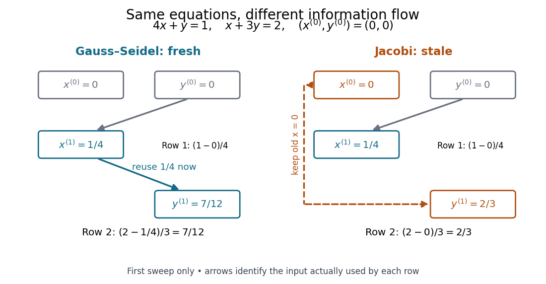
Fresh and stale inputs in the first sweep of the original two-variable linear system
. Details. 
With a stale first coordinate, the Jacobi method would instead give after the first sweep. Both methods have the same fixed point, but changing when coordinates become available changes the entire sequence of vectors.
Work by Gasper J. Piermarini 2026-10-18
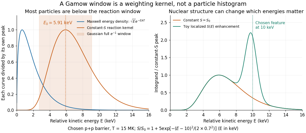
The Gaussian approximation to a nonresonant thermonuclear rate already gives the saddle and curvature. In its notation , so the same result readsThe full width joins the two points at of the peak of the approximating Gaussian function; it is neither its standard deviation nor its full width at half maximum . These are local Gaussian approximation widths, not exact equal-height endpoints of the asymmetric kernel.
Why keep the astrophysical S factor inside the integral? If is positive and smooth, stationarity of gives a leading peak displacement . The slow-variation test is therefore , together with small curvature corrections. More generally any energy-dependent prefactor shifts the saddle; a temperature-dependent prefactor also changes the local temperature exponent of a thermonuclear reaction. A sharp nuclear feature can invalidate this expansion altogether.
Choose and for an illustrative proton pair. Then , and . The relative Maxwell-Boltzmann velocity distribution has energy-density maximum , far below the reaction kernel's maximum. Now choose the deliberately artificial enhancementNumerical integration raises the rate by about at the same temperature, even though the enhancement is away from . This is a sensitivity experiment, not a claimed proton–proton nuclear level or a physical nuclear line-shape model. It illustrates why extrapolating without checking nearby structure can fail.

Proposer-optimal stable matching 2026-10-18
For fixed strict preferences, a proposer-optimal stable matching gives each proposer its best partner obtainable in any stable matching, with unmatched ranked last. The Gale-Shapley algorithm achieves all these individual optima simultaneously. In the worked example, gives partners ranked , respectively; the alternative gives them ranks .
Suppose a first rejection of a pair belonging to some stable matching occurs when rejects for . Every partner prefers to has already rejected it, so none can be its partner in . If , then prefers to , while prefers to : a blocking pair in stable matching, a contradiction. Hence no rejected pair is stable, and each proposer receives its best stable partner. Under strict preferences this also makes the outcome independent of proposal order.
Franck-Hertz spacing fit and contact offset 2026-10-18
Fit the positions of successive, consistently defined troughs by linear regression, . A constant intercept absorbs the contact potential difference, collection phase and initial energy effects; estimates the repeated loss expressed as a voltage. Subtracting successive positions cancels . A line fit uses every position and leaves residuals that can reveal curvature or a misidentified trough. It still assumes that the phase is constant over the fitted range and that all troughs belong to the same loss channel.
For an original numerical example, choose and synthetic positions . Their successive spacings are . The ordinary least squares formulas giveThe fitted residuals are , with zero sum and zero index-weighted sum. Their residual sum of squares is . If independent, equal-variance, zero-mean errors describe these positions, the residual variance estimate is and the slope standard error is . Thus the inferred model loss is with conditional standard error . These errors summarize only the chosen position scatter; a voltage-scale error or a drifting collection phase is not included. Adjacent spacings share a position error and are therefore correlated even when position errors are independent.
The offset has a sharper identifiability limitation. Even if a constant-phase model were exact, an initial beam kinetic energy shifts the troughs by . For the symmetric illustrative curve, . The transformation , leaves every trough position unchanged. Measuring alone therefore cannot determine the contact potential difference. Relabeling also changes by without changing . An independent offset calibration and a justified collection model are needed before turning a first trough into an excitation threshold. Varying tests this model's predicted half-voltage shift of the trough centers; it is a diagnostic prediction of this chosen curve, not a universal correction for experimental minima.
Franck-Hertz repeated-loss collection model Created 2026-10-18 Updated 2026-10-20
Define a signed offset so that the accelerating region adds kinetic energy . This convention concerns this gap; collector contact fields belong in the effective . An electron emitted with initial kinetic energy and undergoing identical excitation losses reaches the grid withEach loss excites a fresh chemical atom initially in its ground state. These are repeated payments of the same excitation cost. The index counts events along an electron trajectory, not the ordinal number of an atomic excited state. The outgoing energy also does not locate the last collision: after an early collision an electron can regain enough kinetic energy to cross the barrier.
At fixed , let be the normalized initial-energy probability density function within the ensemble of electrons reaching the grid, and the conditional probabilities for losses within that ensemble. Then the ideal collection law isTake and exclude paths with insufficient kinetic energy for a loss at its actual collision position. The weights contain collision positions and rates, mean free paths and angular acceptance. This equation is a bookkeeping model, not a derivation of those weights. Multiplying all incident particles by one constant transmission is an additional approximation; real transmission and can vary with .
One analytical extreme assumes , one-dimensional motion and an immediate loss whenever the kinetic energy reaches . With , and , the number of losses and remaining kinetic energy areHere is the floor function. Collection switches off for an interval of width after each reset, then recovers; the pattern repeats every . For , and , an applied gives , and rejection, whereas gives , and collection. With the dips disappear in this idealization. With no collisions, there is only a single collection onset. Both limits expose the separate roles of loss and filtering.
To draw a smooth illustrative curve, extend this periodic rule mathematically to all and convolve it with a chosen normal distribution of voltage jitter, of standard deviation :Here is the standard normal cumulative distribution function. Each summand is the smoothed indicator of the accepted interval . The result satisfies and has period . For the figure choose and plot only well beyond the startup region. This is a chosen phenomenological curve, not a Boltzmann equation transport prediction or a fit to measured electric current. Its symmetric troughs center on , rather than the reset voltages . Finite excitation rates, several loss channels, space charge, initial angular and energy spreads, and real electrode geometry can change the trough shape and phase; a single convolution does not solve these effects.
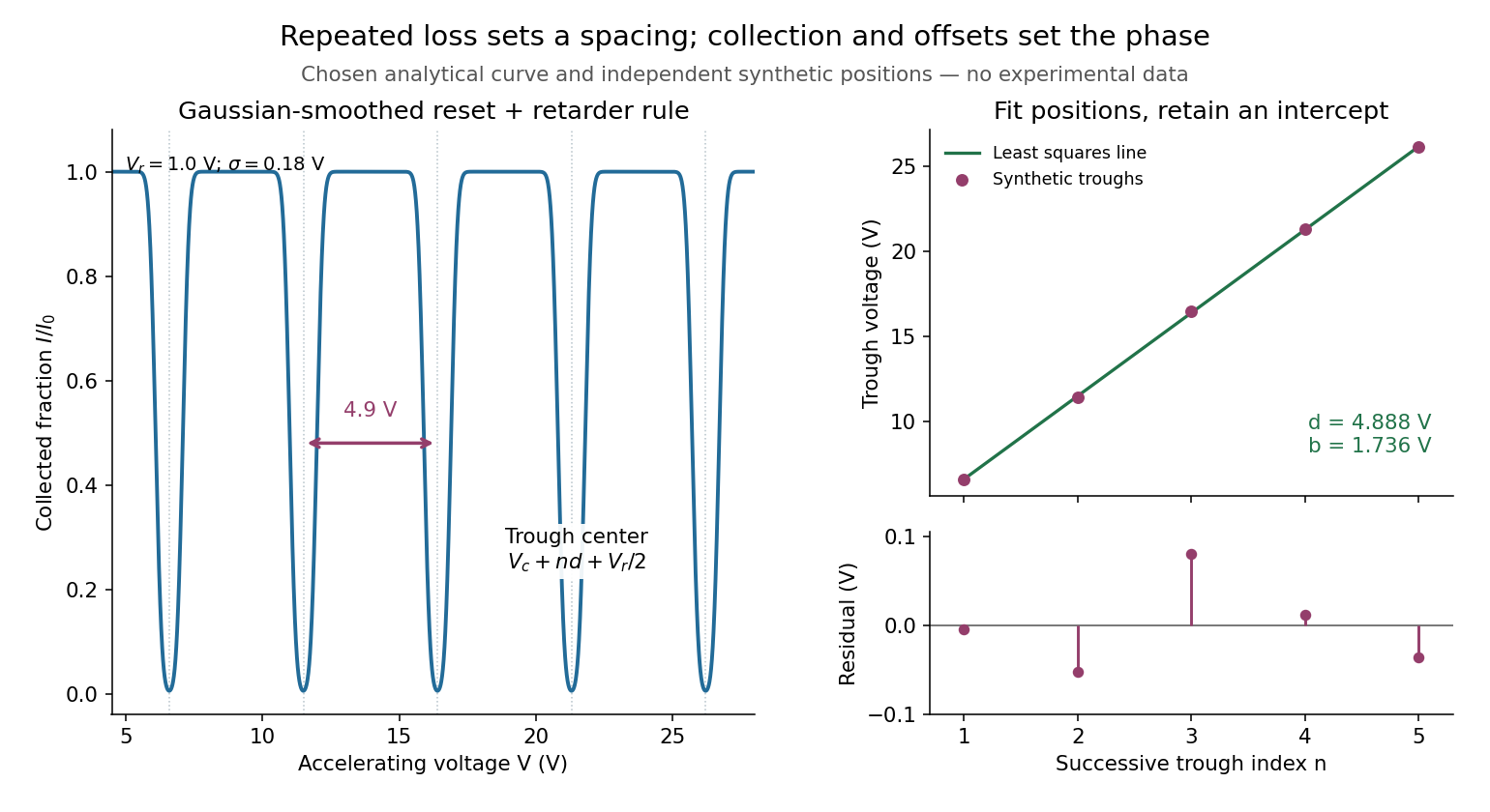
Illustrative repeated-loss collection and an independent synthetic spacing fit
. Left: the chosen Gaussian-smoothed threshold model, with , , and . Right: separately chosen synthetic trough positions, their ordinary least squares fit and residuals. The points are not extracted from the left curve or a historical trace. Source. Details.
Franck-Hertz retarding collector transfer Created 2026-10-18 Updated 2026-10-20
For electrons directed normally toward an ideal planar collector, a retarding electric potential difference imposes the barrier . Write its transfer as , where is the Heaviside step function and the positive elementary charge. Thus a perfectly sharp loss need not produce a sharp drop in electric current: the drop also depends on where the outgoing energy lies relative to the barrier. For an oblique incident electron at angle to the normal, the same planar model instead tests ; angular scattering can change collection even at unchanged total kinetic energy.
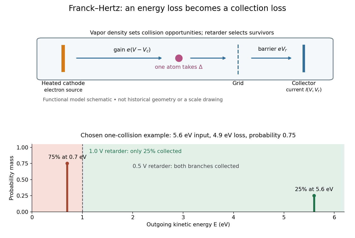
Franck-Hertz energy-loss model: separate acceleration, loss and collection
. Original functional schematic, not a scale reconstruction of a historical tube. The lower panel applies an ideal normally incident retarder to the explicitly chosen one-collision example. Equal vertical strokes mark outgoing energies; their labeled weights give probabilities. Source. Details.
For example, choose a monoenergetic incoming beam with , and . After one encounter, have and have . A retarder collects only , whereas a retarder collects ; here is the incident electric current with fixed geometrical acceptance and no background. The mean outgoing kinetic energy is , independently checked by . These are chosen inputs and calculated fractions, not historical measurements.
More generally, let be the normalized outgoing probability density function at a fixed accelerating electric potential difference , for the normally incident idealization. A retarding scan givesThe second equation follows by differentiating the lower integration limit, with Dirac delta functions understood for sharp beams. It explains why an integrated collector readout can reveal an energy distribution. With angles present it probes the distribution of normal kinetic energy; finite instrumental resolution smooths it, and numerical differentiation amplifies noise. Keep the incoming beam fixed during this scan. A scan of changes itself and cannot be differentiated by the same inversion formula.
Radial Gaussian flat function 2026-10-18
In any finite-dimensional Euclidean space, this extension is a smooth function and all its partial derivatives at the origin vanish. Away from zero, repeated differentiation gives finite sums of coordinate polynomials divided by powers of , multiplied by . Every such term is bounded in absolute value by near zero. Since Gaussian decay dominates every power, this bound tends to zero faster than any prescribed positive power of . Induction using difference quotients then proves smoothness and zero derivatives of every order at zero.
The origin is nevertheless a strict global minimum, because for . All its Taylor series coefficients vanish, so the function is not real analytic at zero. Adding a constant preserves the stationary minimum but changes the zeroth-order value. An expression written only for has no stationary point at the excluded origin until an extension is specified.
Heat bath relaxation with finite capacity 2026-10-18
The equilibrium calculation determines where the two temperatures end, without determining how long they take. Stipulate a constant thermal conductance and the linear heat transfer law underlying Newton's law of cooling. With positive from body 1 to bath 2, the ordinary differential equations areThe dot denotes a derivative with respect to time. This model assumes internal equilibration is fast compared with exchange between the bodies. Adding the two energy rates gives zero; subtracting the temperature rates givesThe temperature difference has exponential decay with time constant . For the finite heat bath example and the stipulated , , and solving the ordinary differential equations givesAt one time constant, , and . Equal temperatures are approached as a limit at infinite time. The finite bath causes the temperature difference to shrink faster than the fixed-bath model, because both bodies change temperature.
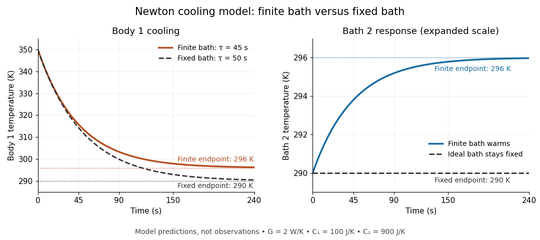
Finite bath and fixed bath Newton's law of cooling histories
. Original analytical model predictions with , and ; time is in seconds. Solid lines show the two finite bodies approaching with time constant . Dashed lines show body 1 cooling toward a bath held at , with time constant . The two panels use different vertical scales so that the finite bath's warming remains visible. Details.
For an ideal heat bath with the same , set rather than evolving its temperature. Newton's law of cooling then yieldsChanging changes these time constants, while the final temperature is fixed by the capacities and initial conditions. The dynamical model independently checks the Second law of thermodynamics:Its integral over the relaxation reproduces the endpoint entropy change. The useful separation is between capacity, which governs how much the bath temperature shifts, and thermal conductance, which governs the exchange rate. Neither alone establishes a reliable heat bath.
Finite weighted geometric sum 2026-10-18
Differentiate the finite geometric series with respect to , then multiply by . This proves the title identity for without any infinite-series differentiation. At , the sum is . For , both and tend to zero, yielding .
Cyclic group of order four 2026-10-18
The cyclic group generated by with and has elements . It is realized by quarter-turn rotations of a plane. The cyclic group of order four and Klein four-group have the same order but different element orders: the latter has no element of order four.
Observation of Fermi pressure in trapped lithium Created 2026-10-18 Updated 2026-10-20
In 2001, Andrew G. Truscott, Randall G. Hulet, and collaborators observed degeneracy pressure in trapped lithium. A Zeeman slower fed a dual magneto-optical trap; optical pumping prepared atoms for a cloverleaf apparatus for magnetic trapping of neutral atoms. Microwave evaporation removed energetic lithium-7 bosons; elastic collisions cooled lithium-6 fermions by sympathetic cooling.[ref]
Observation of Fermi Pressure in a Gas of Trapped Atoms by Andrew G. Truscott and others. Truscott et al., Observation of Fermi Pressure in a Gas of Trapped Atoms (2001), p. 2570, preparation and cooling
Sequential absorption imaging recorded both trapped clouds on a camera. Fits to axial profiles used the boson cloud as a thermometer. At common temperature, the nearly equal magnetic trapping potentials provided a comparison: the clouds had similar sizes near , but the fermion cloud remained broader as cooling reached . Figure 3 compared its radius with ideal Fermi gas and classical predictions.[ref]
Observation of Fermi Pressure in a Gas of Trapped Atoms by Andrew G. Truscott and others. pp. 2570–2572, Figs. 1–3, imaging, thermometry, and radius comparison
Varying the wait before imaging tested thermal equilibrium. Finite imaging resolution restricted the analysis to the axial direction; fits neglected interaction-induced density shifts. Cooling eventually suffered from the dwindling boson heat capacity. The result supports quantum occupation effects, without directly resolving individual occupied states or reaching zero temperature.[ref]
Observation of Fermi Pressure in a Gas of Trapped Atoms by Andrew G. Truscott and others. p. 2571, axial resolution and negligible-interaction approximation; p. 2572, equilibration test and cooling limit
These were neutral alkali atoms in a spatially varying trap. The Fermi energy of a model electron gas instead uses uniform electrons, two equally populated spin states, and the electron mass. The measured trapped-atom radii are not measurements of that electron model's or ; comparing their numerical Fermi energies requires the appropriate particle mass, internal-state populations, and confining potential.
Fermi energy of a model electron gas Created 2026-10-18 Updated 2026-10-20
Choose for a uniform noninteracting electron model with two equally populated spin states. This is an original worked example, not a measured number density assigned to an actual material. Using , , and givesThe conversion uses : an electronvolt is an energy unit, while a joule is its SI counterpart. The dimensions provide a quick check: is inverse length, has units of momentum, has units of energy, and has units of temperature. The ratio verifies the nonrelativistic limit for this model, where is the speed of light.
Increasing this chosen number density eightfold doubles the Fermi momentum and quadruples the Fermi energy, giving approximately . The exponent has a geometric origin: the number of occupied states grows as the cube of a momentum radius, but kinetic energy of nonrelativistic particles grows as its square. This makes Fermi energy a useful bridge between a count of particles and a mechanical energy scale.
Fermi temperature Created 2026-10-18 Updated 2026-11-05
The Fermi temperature expresses a Fermi energy as a temperature scale, , where is the Boltzmann constant. In the convention measured from the relevant band minimum, is the regime of a strongly degenerate Fermi gas. For an interacting Fermi liquid, an effective Fermi scale can be introduced through its quasiparticle dispersion; its convention should be specified.
Faraday rotation in a glass-rod experiment 2026-10-18
A William & Mary teaching experiment places a glass rod inside a solenoid. Align a polarized helium-neon laser through the rod's centre onto a photodiode after a rotatable polarimeter analyzer. First scan the analyzer from maximum to minimum transmission in steps and record detector voltage, establishing the angular response. A function generator and electronic amplifier then drive sinusoidal electric current through the solenoid; a multimeter measures the electric current and an oscilloscope reads the photodiode. Trigger the oscilloscope from the generator, remove the large constant detector component by AC coupling, and average repeated traces. Convert the small synchronized voltage modulation to rotation using the calibrated angular slope. The manual fits rotation against magnetic flux density, using its stated coil calibration and converting measured root mean square current to peak current. This is a specified laboratory procedure, rather than measured results reproduced here.[ref]
Faraday Rotation. Physics 251: Experimental Atomic Physics, Fall 2019; William & Mary, Faraday Rotation laboratory chapter: printed pp. 2–7, apparatus, alignment, analyzer calibration, synchronized readout and equations (1.8)–(1.9)
To test the inference, add matched zero-electric current readings before and after each reversal, hold the analyzer fixed during paired readings, and compare equal positive and negative electric currents. A blocked beam tests electrical pickup in the detector channel. These are proposed controls. Joule heating scales as current squared, so reversing electric current at equal magnitude helps separate an odd rotation from even heating effects; it does not remove drift between readings. Record temperature and allow repeatable settling. Changes in transmission, mechanical motion, stressed-glass birefringence and detector pickup can imitate a signal. Synchronized averaging suppresses unsynchronized noise, but cannot reject an artifact synchronized to the drive.
Quantitative extraction of the Verdet constant also needs the integral of magnetic flux density through the rod: a finite solenoid can have a nonuniform axial magnetic field. Use its calibrated path integral, or justify a uniform-field approximation; do not silently multiply a central field by the whole rod length. A signed reversal or phase-sensitive readout tests the part odd in applied magnetic field. Its agreement with the simple rotation law supports the model under these controls, rather than proving that every change of transmitted light intensity is Faraday rotation.
Consider an original model at fixed vacuum wavelength and temperature . Stipulate a transparent sample with Verdet constant , length , uniform adjustable , and a field-independent analyzer-zero offset . These are chosen values, not measured glass properties. On a continuously tracked small-angle branch,Taking half the difference gives ; half the sum recovers . Hence . A field-reversal difference of is twice the single-field rotation, not that rotation itself. More generally this subtraction removes every contribution that is even under , provided the sample and apparatus remain otherwise matched.
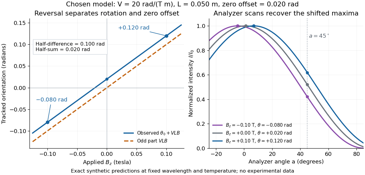

An ideal polarimeter analyzer at laboratory angle reads normalized light intensity . Here is the light intensity immediately before the analyzer, separately calibrated for each condition. A scan locates the maximum at modulo . At , expansion about zero gives , with angles in radians. At crossed extinction, the response instead begins as and loses the sign near zero. The favorable slope follows directly by differentiating Malus's law; its sign reverses if the angular convention is reversed.
There are unlisted articles, also show them or only show them.