
Faraday rotation on a round trip 2026-10-18
Faraday rotation exhibits optical nonreciprocity: with the bias magnetic field held fixed, a retracing beam gains another rotation in the same laboratory sense. Natural optical activity in a reciprocal medium instead unwinds on retracing the path.[ref]
Faraday effect. RP Photonics Encyclopedia, Faraday Effect, Rüdiger Paschotta: What is the Faraday Effect?, doubled rotation on a round trip
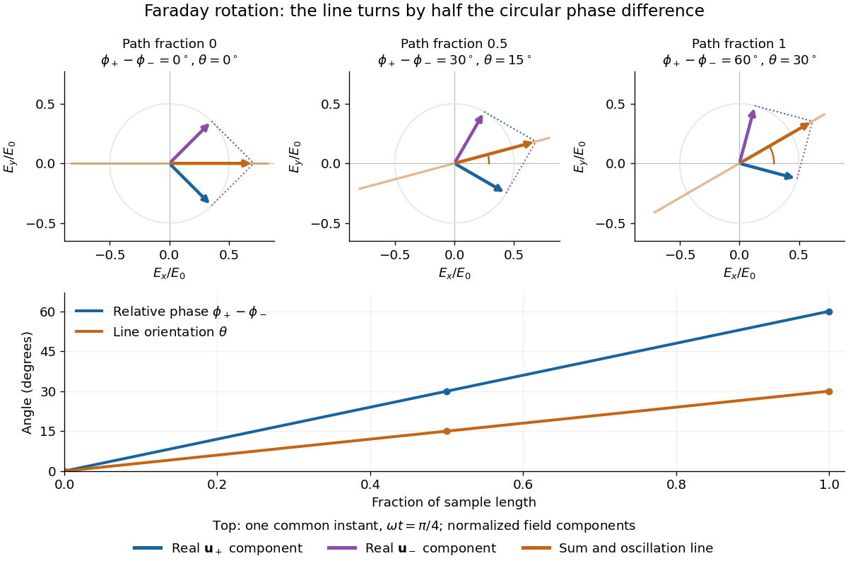
To reconcile this with the signed formula, retain the laboratory axes for comparing physical lines. For the backward ray choose a right-handed ray basis , , . Its magnetic flux density component is , so its local rotation increment is . But positive is negative laboratory : the backward increment is therefore in the laboratory orientation plot. Reversing the ray reverses both the longitudinal component and the basis used for its signed angle. Reversing only one creates the false prediction of cancellation.
In fixed laboratory transverse components, define the rotation matrixFor an ideal mirror at normal incidence that contributes the same complex amplitude factor to both transverse components, the round-trip map is . The common mirror factor does not change the oscillation line. A reciprocal natural rotator instead gives . This comparison assumes a retraced straight path and no additional polarization-changing elements.
For example, a chosen single-pass Faraday rotation produces a returned line at to the original laboratory axis. A chosen reciprocal natural rotator returns it to . The same addition makes an ideal optical isolator possible: polarizers at and surround a Faraday rotator. Forward light follows and passes. Returning light selected at reaches at the entrance polarizer and is rejected by Malus's law. Real transmission loss and incomplete extinction limit the isolation.
Faraday rotation from circular phases 2026-10-18
The factor of one half follows from superposition, without assigning ambiguous right/left names to the circular polarizations. Use the complex amplitude convention and fixed transverse unit vectorsFor equal transmitted wave amplitudes, let the accumulated wave phases be and . Their sum isThe common wave phase sets the timing of the electric field oscillation; the real direction in parentheses sets its linear polarization. Opposite circular polarizations have changed their relative wave phase, yet their sum still oscillates along a line. Unequal transmitted wave amplitudes would generally give elliptical polarization instead.
In a uniform sample, with refractive indices and vacuum wavenumber , the phase difference is . ThusThe second relation identifies the small signed circular birefringence responsible for the rotation in this basis. Unlike a waveplate, whose separated modes have orthogonal linear polarizations, this ideal rotator has modes with opposite circular polarizations.

Verdet constant 2026-10-18
The Verdet constant is the coefficient relating Faraday rotation to the magnetic flux density path integral. Its SI units are . It depends on material, wavelength and temperature; a sign requires the stated viewing convention.[ref]
Faraday effect. RP Photonics Encyclopedia, Faraday Effect, Rüdiger Paschotta: What is the Faraday Effect? and Verdet Constants of Materials
The name commemorates Émile Verdet. For nonuniform material or temperature, use when the local scalar description remains valid. A single central magnetic field reading cannot generally replace this weighted integral. Strong additional linear birefringence or appreciable circular dichroism requires following the full polarization of an electromagnetic wave, rather than treating the output as merely a rotated line.
For a positive integer , multiply the exponential series by and integrate term by term from zero to . Its uniform convergence on every compact interval justifies the operation and proves the title identity. The resulting power series converges absolutely for every real or complex , by the ratio test. Repeated integration by parts evaluates the right side as an exponential times a polynomial, with its constant chosen to make the integral vanish at zero.
For an action , vary the field with compact support, or fix both and its first derivatives on the boundary. One integration by parts on the first-derivative term and two on the second-derivative term give the displayed Euler-Lagrange field equation. With ordered repeated indices, define the second-derivative coefficient symmetrically so that . This convention avoids an unintended factor of two in mixed derivative terms. Higher spatial derivatives alone do not require higher time derivatives.
Damped and antidamped fields from an antisymmetric velocity coupling Created 2026-10-18 Updated 2026-11-05
Adding to the cross-coupled scalar Lagrangian density produces independent equations and . For the convention , their frequencies are respectively and . Above the threshold they oscillate with decaying or growing envelopes; below it they have nonoscillatory real temporal exponents. At equality the repeated temporal root supplies . At each equation also has a constant solution. The full system is generically unstable because of the amplified second field, even though it arises from an autonomous variational system with conserved, indefinite total energy.
History of Euler characteristic 2026-10-18
Leonhard Euler's Elementa doctrinae solidorum, or Elements of the doctrine of solids, appeared in 1758 in volume 4 of Novi Commentarii academiae scientiarum Petropolitanae, pp. 109–140. The repository record dates its composition to 1750. Composition and publication are distinct dates here.[ref]
The modern cell-count formula for Euler characteristic puts polyhedral counting into an arbitrary-dimensional CW complex. It also identifies what is being counted: the Euler characteristic of a cube boundary and its interior distinguishes a polyhedral surface from the filled solid using the missing three-dimensional term. The modern homology formulation explains why this alternating arithmetic persists across different decompositions.[ref]
Algebraic Topology by Allen Hatcher. Algebraic Topology by Allen Hatcher, §2.2, printed pp. 146–147, Theorem 2.44: alternating cell counts, homology ranks and independence from the CW structure
For a concrete example of cellular homology of real projective space, the real projective plane has one topological cell in each of dimensions zero, one and two. Its one-dimensional topological cell is a loop, and the face attaches around that loop twice. Choose orientations so that the cellular chain complex over the integers iswith nonzero chain groups in degrees two, one and zero. The twice-around attachment is why the first boundary operator shown is multiplication by two.[ref]
Algebraic Topology by Allen Hatcher. Algebraic Topology by Allen Hatcher, §2.2, Example 2.42, printed p. 144: real projective cellular boundary maps
Over the rational numbers, multiplication by two is invertible, so and vanish, while . Over the finite field , two equals zero. Both boundary operators then vanish, giving one-dimensional homology groups in all three degrees. Their respective Betti numbers areNevertheless,The direct cell count is also .
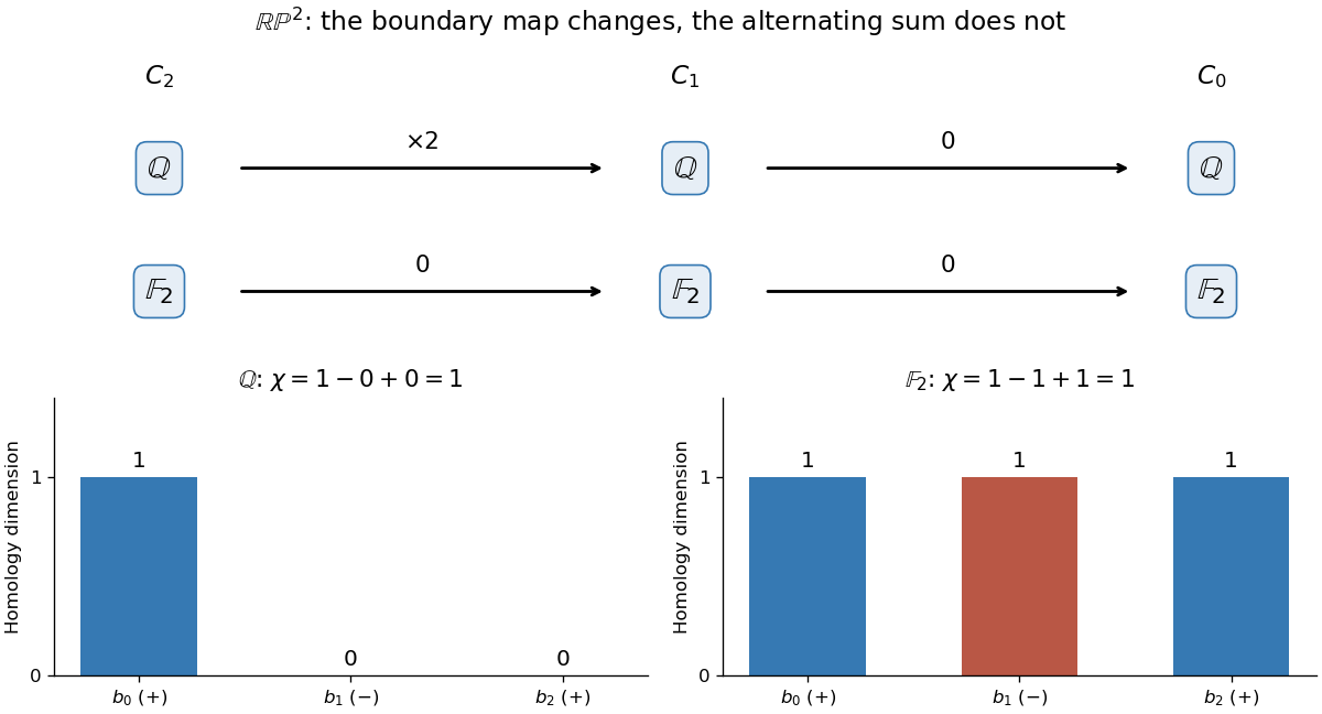
Changing coefficients changes the projective plane's homology groups, but their alternating dimension sum remains 1
. Details. 
This calculation makes the strength and loss of information visible. The Euler characteristic survives a change of the field used for coefficients, while individual homology groups can change. Over the integers, the same chain complex has and : a torsion subgroup that rational Betti numbers do not record. The rank cancellation in the Euler-Poincare formula explains why the alternating total still agrees with the cell count.
The boundary of a cube has eight vertices, twelve edges and six square faces. Treating each open face as a two-dimensional topological cell givesThis agrees with its being a two-sphere: stretching the hollow polyhedral surface changes its geometry but not its topology. The interior is excluded from this space.
Now include the solid interior. The cube has the same lower-dimensional topological cells, together with one open three-dimensional topological cell. The cell-count formula for Euler characteristic becomesThe filled cube is contractible, so its homology agrees with that of a point. The term is essential: by itself is the full count only for a two-dimensional CW complex.
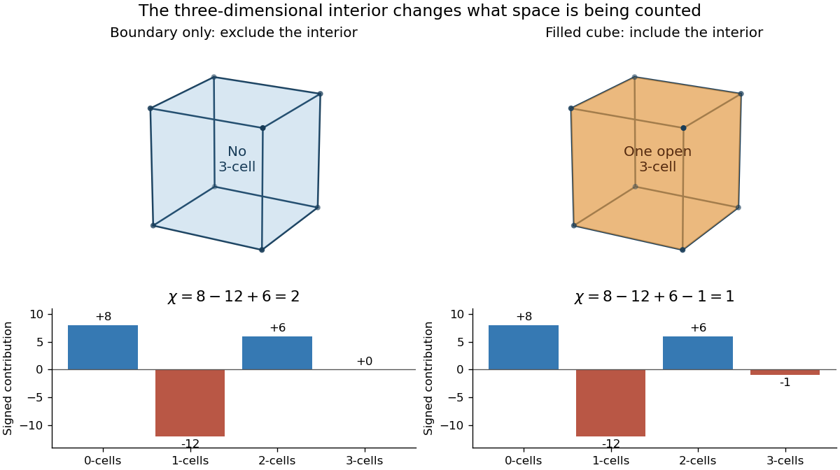
The boundary of a cube has Euler characteristic 2; including its three-dimensional interior adds one negative contribution and gives 1
. Details. 
Adding a diagonal within one square face replaces that face by two triangular faces and introduces one edge. Thus the Euler characteristic changes by , as in subdivision invariance of Euler characteristic. Including an interior is a different operation: it adds points to the space, rather than giving the same space a finer description. This distinction matters whenever a geometric model could mean either a surface or the solid it encloses.
If the variable-site model counts every sector with weight , its exact relative partition sum is . Differentiating its logarithm gives the displayed exact mean. Minimizing the leading extensive Gibbs free energy instead gives , the same result to relative order . Its exact relative equilibrium free energy is . This correction distinguishes a thermodynamic saddle from an exact finite-system average; changing the microscopic site-creation convention can also change subextensive factors.
Fix a failure probability and assume an independent and identically distributed statistical sample. A finite-sample confidence band for its population cumulative distribution function isHere is the natural logarithm. The DKW inequality impliesThis is simultaneous coverage over the whole real line, valid at each fixed sample size.[ref]
To obtain the band, solve for the positive . Outside a failure event of probability at most , for every . Since a cumulative distribution function already lies in , clipping the endpoints to this interval preserves the coverage event. The guarantee is at least , and need not equal it.
Choose , giving at least simultaneous coverage under the stated model. For , respectively, the half-widths before clipping areFor the chosen five observations, the band at is , while at it is approximately . At the unclipped band would be , so clipping gives . The broad uncertainty is informative: five observations give a precise description of themselves, but a coarse bound for an unknown population cumulative distribution function.
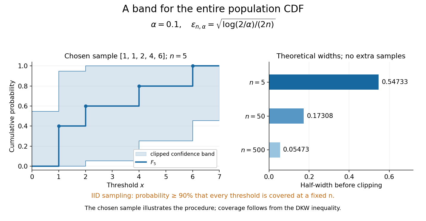
Finite-sample simultaneous uncertainty around an empirical distribution function
. Left: the chosen five observations give and its band clipped to , using . Right: theoretical half-widths for , with no additional samples constructed. The confidence band has coverage at least under independent and identically distributed sampling; the drawing illustrates the procedure and does not establish its coverage. Details.
A collection of pointwise confidence intervals only promises coverage separately at each preselected threshold; it does not promise coverage of an entire cumulative distribution function. Here the one simultaneous event permits inspecting any threshold after seeing the data. The probability refers to repeated sampling of the entire statistical sample, with fixed. It does not assign probability to a fixed after observing this particular band, and it is not a prediction interval for a future observation. The displayed comparison gives a guarantee for each fixed separately, not simultaneous validity over all sample sizes or an optional stopping rule. The chosen observations are an illustration; the coverage claim follows from the DKW inequality, not from their appearance or a simulation. Dependence or observations with different sampling laws require another argument.
At fixed , multiplying by divides the half-width by . Conversely, a desired half-width is ensured by , rounded up to an integer. For and , this sufficient sample size is . This makes the confidence band useful for planning how many observations are needed before estimating threshold probabilities to a chosen simultaneous accuracy.
Dvoretzky-Kiefer-Wolfowitz inequality 2026-10-18
For independent and identically distributed real random variables with cumulative distribution function , the Dvoretzky-Kiefer-Wolfowitz inequality gives, for every and ,The supremum is the Kolmogorov distance: a single event controls all thresholds simultaneously. The bound holds for discrete, continuous, and mixed probability distributions.[ref]
For one fixed threshold, Hoeffding's inequality gives the same expression as an upper bound on . That fixed-threshold result alone does not justify moving the supremum inside the probability. The DKW inequality is the stronger statement needed for a simultaneous empirical distribution confidence band.
Thermal-shell estimate of electronic heat capacity Created 2026-10-18 Updated 2026-11-05
For a three-dimensional free electron model, the spin-summed density of states at the Fermi energy is . A shell estimate treats electrons as thermally active and assigns each an excitation energy of order . For the illustrative choice , and differentiation gives . The numerical coefficient is heuristic: the controlled Sommerfeld expansion instead givesBoth estimates express Pauli exclusion principle suppression of the classical heat capacity when . A shell argument establishes scaling rather than a universal prefactor.
Proton-motive force 2026-10-18
A proton-motive force is a proton electrochemical potential difference per unit electric charge. It combines the electric potential difference and the chemical potential difference across a cell membrane; the direction and sign convention must be specified.
Negative differential resistance 2026-10-18
A local negative slope of a current-voltage characteristic, where the inverse slope exists. This differs from negative : a tunnel diode can have positive electric potential difference and positive electric current while .
Magnetoresistance Created 2026-10-18 Updated 2026-10-20
A change of electrical resistance associated with an applied magnetic field, with material, temperature, measuring electric current and preparation specified. The response can depend on magnetic history as well as the instantaneous field. A magnetoresistance measurement therefore compares defined states, rather than treating every material as a single-valued function of field magnitude.
Siemens (unit) Created 2026-10-18 Updated 2026-11-05
The siemens, symbol , is the SI unit of electrical conductance and electrical admittance: . A conductance of corresponds to resistance for an ideal resistor.
The same unit can describe a complex electrical admittance in a sinusoidal experiment; that value includes a reactive part as well as conductance. For a uniform conducting sample, electrical conductivity instead has units because the conversion from material response to conductance also involves sample area and length.
Photoelectric threshold frequency Created 2026-10-18 Updated 2026-11-05
The photoelectric threshold frequency is the lower frequency boundary allowed by the ideal single-photon energy balance. With vacuum wavelength and speed of light , its corresponding longest wavelength is . The chosen work function gives and . These are model parameters, not a measured threshold for a named metal. Detectable photocurrent need not begin abruptly at the ideal boundary: collection, finite spectral width, thermal broadening and surface inhomogeneity matter.
Dummy index 2026-10-18
A dummy index is summed over its full specified range. Its name can be changed consistently without changing the expression, as in . A free index specifies a component and cannot be renamed in only one term of an equation. Relabelling dummy indices is useful for tensor contraction arguments involving a symmetric tensor and an antisymmetric tensor.
Rubbery plateau Created 2026-10-18 Updated 2026-11-05
The rubbery plateau is a frequency or time range in which a flexible polymer network has an approximately constant elastic storage modulus dominated by chain entropy. A permanently crosslinked elastomer retains a nonzero long-time modulus. An entangled uncrosslinked polymer melt can have a transient plateau but ultimately reaches terminal fluid flow at sufficiently low frequency. The plateau therefore must be interpreted with the network lifetime and observation window specified.
There are unlisted articles, also show them or only show them.