
Kruskal's algorithm worked example 2026-10-18
Consider this original connected graph on vertices . Its undirected edges, already in increasing weight order, areHere means the unordered pair ; the weights are dimensionless costs. Accept and , with total . Reject : its endpoints already have the graph path , so it would close the graph cycle . Accept and , reaching all five vertices with four edges. The resulting minimum spanning tree isStop here: and need not be examined. If processing continued, both would be rejected because their endpoints are already in the same connected component of a graph.
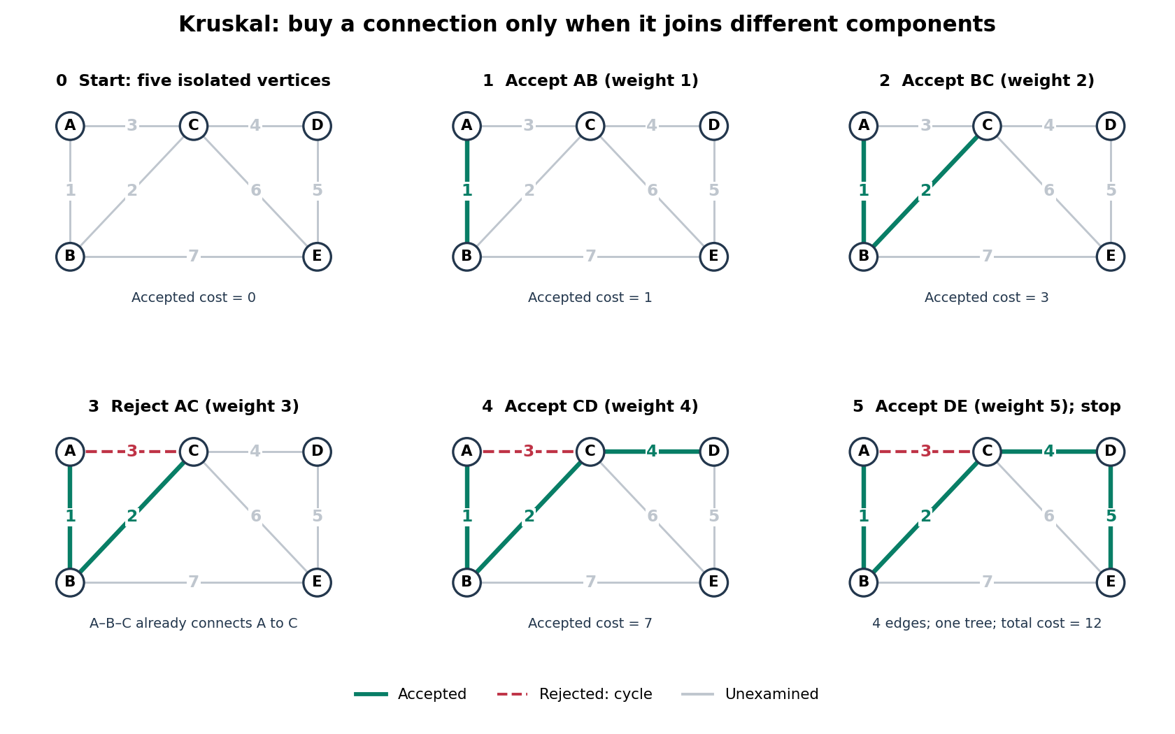

Taking the three cheapest edges instead gives a graph cycle on , leaving isolated: it is neither a forest nor a spanning tree. Even taking the four cheapest edges adds only and leaves isolated. A cheap infeasible selection cannot compete with a minimum spanning tree. For this small graph, checking all four-edge subsets gives a direct certificate: among those that are spanning trees, exactly one has minimum cost , namely . The general algorithm avoids this exhaustive search.
Kelvin-Voigt rod Green function Created 2026-10-18 Updated 2026-11-05
For a rod with unit mass density and elastic modulus, the Kelvin-Voigt model gives , . For the operator with the opposite overall sign, , the inverse under the Fourier transform convention is the displayed expression. Its poles are . With real, the retarded fundamental solution in spatial Fourier variables is . Its initial derivative is , fixed by the leading coefficient . At a repeated root take the continuous limit; for imaginary the sine becomes a hyperbolic sine.
The physical Jeans length is . A pressureless uniform sphere of initial density has free-fall time of a uniform sphere , giving the title relation. Thus a full-wavelength sound-crossing time and this exact free-fall convention agree in scaling, not numerical value. Using the scale instead gives , the inverse long-wave static Jeans growth-rate spectrum limit. At the threshold itself pressure balances gravity and the net growth rate vanishes; the pressureless free-fall time must not be confused with that marginal mode's infinite growth time.
A strictly diagonally dominant matrix guarantees convergence of the Jacobi method for every initial vector.[ref]
Notes for Ma221 Lecture 21, Nov 10 2009. Math 221, Matrix Computations, Fall 2009; Theorem 1 on strict row diagonal dominance and its proof beginning “Split A = D − (D − A)”
Indeed, using the maximum norm , the induced operator norm is the largest absolute row sum. The Jacobi method has and for , soThis gives a cheap sufficient check without computing any eigenvalues. For the Jacobi iteration for a three-variable tridiagonal system, the absolute row sums of are , giving . The true spectral radius gives a sharper eventual rate.
Strict diagonal dominance is sufficient, not necessary: violates it in the first row, but its Jacobi method has eigenvalues and converges. Conversely, being a positive-definite matrix alone is insufficient: the Jacobi convergence for a three-by-three equicorrelation matrix with has positive eigenvalues for , but spectral radius for its iteration matrix. The extra tridiagonal matrix structure in Jacobi convergence for a symmetric positive-definite tridiagonal matrix is therefore substantive.
Consider the original linear system with a symmetric matrix that is also a tridiagonal matrix:Here and the Jacobi method readsStarting from , the first three vectors areEvery right-hand side uses superscript , including the middle row, even when a new first coordinate has already been computed.
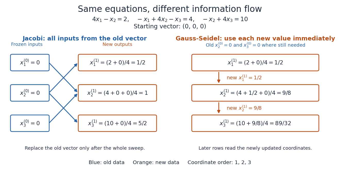
Simultaneous old-to-new component updates in the Jacobi method, compared with immediate reuse in the Gauss-Seidel method
. Details. 
For comparison, a first Gauss-Seidel method sweep in coordinate order givesThe new first coordinate enters the middle update, and the new second coordinate enters the final update. Accidentally overwriting old coordinates during a Jacobi method sweep therefore changes the mathematical method.
The linear-system residual is computable without knowing . The forward error is the actual difference from the desired solution. For an invertible matrix,Keeping fixed, the approximate vector exactly solves with . Thus, for , is the relative backward error when only the right-hand side may change. For a vector norm and its induced operator norm,A small relative linear-system residual ensures a small relative forward error when the condition number is moderate; an ill-conditioned matrix can amplify it. The bound follows directly from and .[ref]
2.8 Conditioning of linear systems. Fundamentals of Numerical Computation by Tobin A. Driscoll and others; §2.8.1, Theorem 2.8.1, equation (2.8.6), right-hand-side perturbation bound applied with Δb = −r
For the Jacobi iteration for a three-variable tridiagonal system, the first linear-system residual is , while the first forward error is . In the Euclidean norm, the relative forward error is and the relative linear-system residual is . Its spectral condition number of a positive-definite matrix is , so the bound is about . The bound is a guarantee, not an equality. In floating-point arithmetic, recompute the linear-system residual from the current vector when checking termination; a small update alone need not certify a small forward error.
A stationary iterative method for a linear system converges to its specified fixed point for every initial vector if and only if its iteration matrix satisfies , where the spectral radius is the largest modulus of an eigenvalue.[ref]
Notes for Ma221 Lecture 21, Nov 10 2009. Math 221, Matrix Computations, Fall 2009; Basic iterative methods: theorem following the spectral-radius lemmas, before the Jacobi update
For a diagonalizable matrix, write . Then , so each eigenvector coefficient tends to zero exactly when its eigenvalue has modulus less than one. For a general matrix, the Jordan normal form gives the same result: a Jordan block with a nilpotent matrix of size satisfiesIf , every coefficient tends to zero because exponential decay beats any fixed polynomial in ; if , the block vanishes once . Conversely, an eigenvector with provides an initial error that cannot tend to zero. For a real matrix with complex eigenvalues, the same obstruction appears in the real invariant subspace spanned by the real and imaginary parts of an eigenvector.
The words "every initial vector" matter. For example, fails the criterion, but still tends to zero. Here a generic initial error has a nonzero first coordinate and diverges; the exceptional errors lie on the second coordinate axis. With , generic errors oscillate rather than diverge in norm, while the same exceptional axis still converges. Both are valid matrix splittings with and . In general the convergent errors form the direct sum of the generalized eigenspaces for ; if , this is a proper linear subspace.
A small spectral radius describes eventual convergence, but does not imply that the Euclidean norm of the error decreases on every step for a non-normal matrix. An operator norm bound does give the stepwise estimate . For a real symmetric matrix, the matrix 2-norm equals its spectral radius, making this particularly direct.
Isotropic fourth moment of a ball 2026-10-18
Here is the volume of the unit ball in -dimensional Euclidean space. Rotational invariance makes the integral an isotropic tensor, while complete symmetry in its four indices equates the three coefficients. Contracting and gives times their common value. The same contraction of the integral is , proving the formula. For the coefficient is . This is the fourth-order counterpart of the isotropic second moment of a ball.
Isotropic rank-three tensor and reflections Created 2026-10-18 Updated 2026-11-05
In three-dimensional Euclidean space, a rank-three tensor invariant under every proper rotation is a scalar multiple of the Levi-Civita symbol. The distinction between proper rotations and all orthogonal transformations matters: . A polar tensor of odd rank invariant under every orthogonal transformation must vanish, since the transformation changes its sign. A nonzero invariant rank-three object under reflections is instead a pseudotensor, whose transformation law includes the extra determinant factor.
For steady Isothermal Bondi accretion from gas at rest at infinity, define , and , where . The Bernoulli function and mass conservation give . The left side has minimum at , and the radius-dependent part on the right has minimum two at . Existence over all positive radii therefore requires the displayed bound. Equality permits the smooth accelerating-inward transonic branch and gives the usual isothermal Bondi accretion rate. Smaller positive rates have an everywhere-subsonic reservoir-connected branch, and zero rate gives a hydrostatic atmosphere. An absorbing inner boundary inside the sonic radius selects the critical inflow; steady isothermal equations and the outer density alone do not specify that inner condition.
Isobaric analog state Created 2026-10-18 Updated 2026-11-05
Nuclear quantum states in different nuclear isobars belonging to the same isospin multiplet, with equal total isospin and approximately the same spatial and spin structure. An isospin raising or lowering operator connects the states in the limit of exact isospin symmetry. Nuclear Coulomb energy and other isospin-breaking effects shift their energies and modify this ideal relationship.
Two-pion isospin decomposition Created 2026-10-18 Updated 2026-11-05
Two pions, each of isospin one, have a nine-dimensional charge-state space. Clebsch-Gordan coefficients decompose it into an isospin-two quintet, an isospin-one triplet and an isospin-zero singlet. Under exchange of the two particle slots, the states are symmetric and the states are antisymmetric. Because pions have zero spin and obey bosonic exchange symmetry, the two-pion channel requires odd relative orbital angular momentum, while require even orbital angular momentum.
Invariant-mass resolution 2026-10-18
The simulation separates a stipulated physical distribution from measurement broadening. Its Cauchy distribution is only a convenient resonance-shaped input, not a complete quantum scattering model. Spatial resolution, magnetic field calibration, Multiple Coulomb scattering, stopping power and incorrect daughter identities all propagate into the measured invariant mass. Instrumental broadening must be understood before interpreting an observed width as a lifetime.
Selection also changes the shape. A momentum threshold can remove low-invariant mass pairs; a fit that fixes the candidate parent's mass would artificially concentrate that same mass and cannot supply an independent search distribution. Compare accepted simulated events with the input distribution, vary justified selection criteria, and check neighboring invariant mass intervals. A peak supported only by one untested selection is weaker evidence than a structure that survives calibration and background checks. The smooth background in the figure is a stipulated control component, not a claim that every physical background is smooth.
Simulated two-track invariant-mass example 2026-10-18
Take two stipulated oppositely charged daughters with equal rest mass and exactly opposite momenta of magnitude . Their total momentum is zero, soThis is a constructed event, not an identification of a historical particle. Boosting both four-momenta by along the first daughter's direction gives total energy and total momentum . Substitution recovers the same invariant mass, although the laboratory energy has increased.
The following independent simulation stipulates 700 signal combinations from a Cauchy distribution centered at with scale , truncated to , plus 2400 background combinations whose density decreases linearly across that interval. Each combination is converted to a back-to-back two-daughter event with . Independent isotropic directions are chosen, each Cartesian momentum component receives normal distribution noise with standard deviation , and invariant mass is reconstructed from the perturbed momenta. All inputs and counts are invented. No historical experimental points or fitted historical parameters appear.
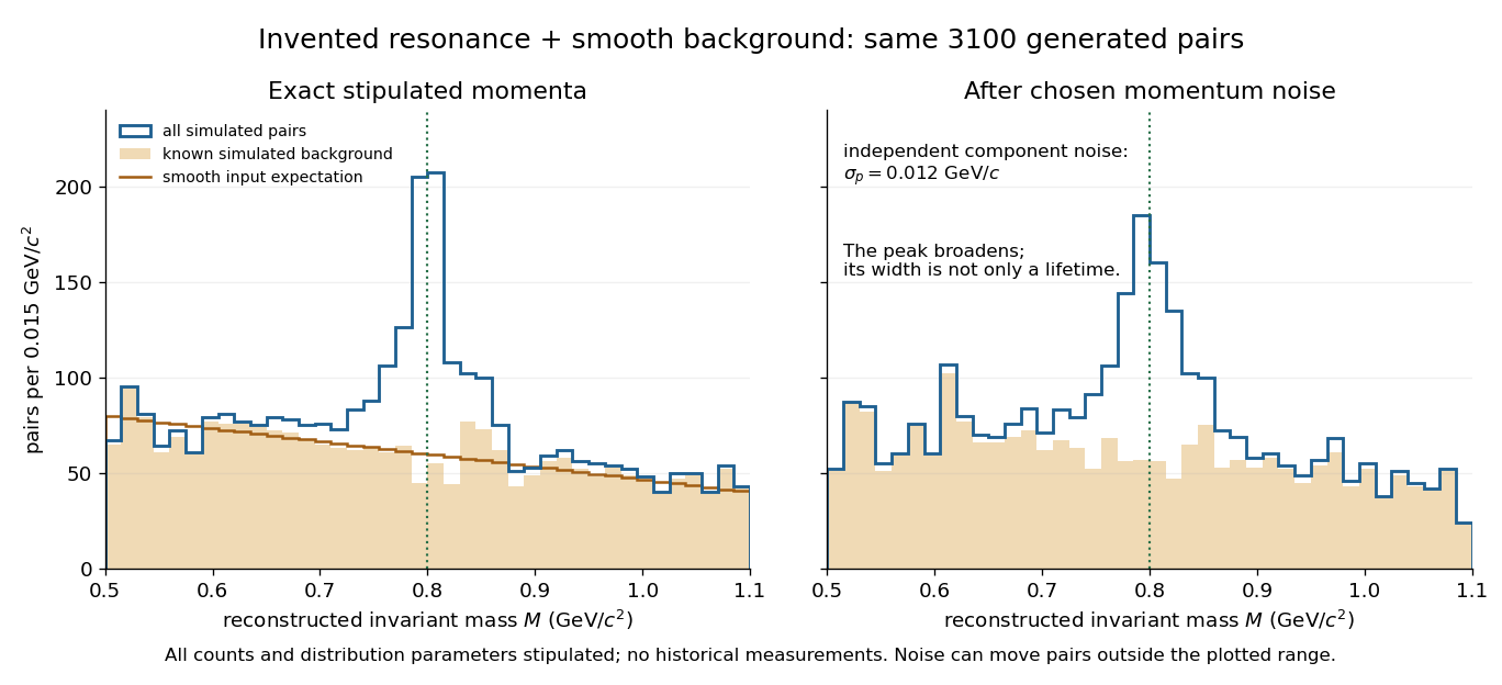
A stipulated resonance component produces an excess above a smooth simulated invariant-mass background
. Original simulation of two-daughter events, with invented counts, a truncated Cauchy signal and a linearly falling background. The two panels share the same generated events. The right panel adds chosen momentum noise before reconstructing invariant mass; this is not an experimental discovery plot. Details.
For torque-free rotation, total angular momentum magnitude and rotational kinetic energy are conserved. Near rotation about principal axis three, eliminate from to obtain the displayed energy difference from . If is largest, it is a constrained energy minimum; if smallest, a maximum. Both extrema are stable in the conservative problem. An intermediate moment gives opposite signs in the quadratic form, a saddle and instability. Dissipation changes the fixed-energy argument and must not be silently added to torque-free motion.
Trigonometric substitution 2026-10-18
A trigonometric substitution is integration by substitution using a trigonometric function to simplify an integrand, especially a square root. For example, , with and , changes to and to . The interval restriction fixes the sign of the square root. Similarly simplifies . The transformed integral must include the differential and, for a definite integral, the new limits.
Charge-induced dipole attraction 2026-10-18
A neutral isotropic atom with static electric polarizability in the field of a distant point charge has induced dipole and energy . Since ,The negative radial force is attractive for either sign of . Reversing reverses the induced dipole but not the energy or leading force. The factor accounts for the work of inducing the dipole; using the permanent-dipole energy without that work would double the answer. The approximation assumes weak fields, a slowly varying field across the atom and negligible electronic overlap.
A localized orbital with two electron spin states has energies , and . Its zero-temperature equilibrium occupation minimizes , where is the chemical potential. For repulsion , the occupation is successively as crosses and . For attraction , the singly occupied state is never the minimum: the occupation jumps from to at . Exactly at a crossing the ground-state occupation is not unique.
At positive temperature, its grand canonical partition function is , where . The expected value of the occupation follows by differentiating: . The factor two counts the two singly occupied microstates, not an additional pair state.
Integrable singularity 2026-10-18
A function has an integrable singularity at a point if it becomes unbounded there but its absolute value has a finite improper integral over a sufficiently small surrounding interval, one-sided at an endpoint. The endpoint behavior of the arcsine distribution's probability density function is an example.
Orthogonality to the image of a matrix 2026-10-18
For a real matrix and a fixed vector , every vector in the image of a linear map defined by is orthogonal to exactly when . Indeed, . If this vanishes for every , choose to obtain . Equivalently each column of is orthogonal to . Requiring the statement only for nonzero changes nothing, since the zero input already has zero dot product. This is the orthogonal complement relation between the image of a linear map and the kernel of a linear map defined by its transpose.
There are unlisted articles, also show them or only show them.