
In dimensions, isotropic modes with dispersion have density of states proportional to . Their equilibrium number is not conserved, so the excitation chemical potential is zero. Integrating and rescaling by gives the displayed energy power and heat capacity proportional to . In three dimensions, linear acoustic phonons give energy and heat capacity; quadratic gapless ferromagnetic magnons give energy and heat capacity. A gap changes the asymptotically low-temperature law to activated behaviour. The mode approximation applies below the relevant band cutoff and when interactions between excitations are negligible.
Born statistical scattering interpretation Created 2026-10-18 Updated 2026-10-25
The scattering interpretation connects an incoming preparation to the relative frequency of outgoing directions and final atomic states. Max Born's 1926 paper treats a distant incoming electron and a chemical atom, expands the outgoing wavefunction into final atomic states, and imposes conservation of energy. Its translated correction footnote specifies the square of the coefficient; the modern complex modulus notation below is ours.[ref]
Zur Quantenmechanik der Stoßvorgänge by Max Born. Zur Quantenmechanik der Stoßvorgänge, 1926, pp. 863–867; inspected in D. H. Delphenich's translation, pp. 2–4, especially p. 3 equation (1) and footnote 1: squared coefficient
In his 11 December 1954 lecture, Max Born recalled the difficulty of interpreting bound electrons alone. He instead described an incident electron wave generating an outgoing spherical wave, with direction-dependent squared amplitude determining relative scattering probabilities. Distinct final atomic states describe excitation with corresponding electron energy loss. This is a retrospective account of an interpretation, rather than the report of a new apparatus.[ref]
The statistical interpretation of quantum mechanics by Max Born. The statistical interpretation of quantum mechanics, lecture delivered 11 December 1954, printed pp. 261–262; inspected through the transcription at studyres.com/doc/8624145/the-statistical-interpretation-of-quantum-mechanics, paragraphs from the bound-electron difficulty through inelastic scattering
The distinction from the modern Born rule matters. The historical question was which collision outcome occurs: a direction of motion and a final atomic state. The general projective measurement formula applies to arbitrary observables, including degenerate outcomes and mixed states; a positive operator-valued measure describes still more general detector statistics. Those formulations should not be read back as the explicit contents of the short 1926 scattering paper. Nor does the scattering interpretation itself supply a rule for the conditional post-measurement state.
Actual experimental settings are described in the Davisson–Germer experiment and the Franck-Hertz experiment. The former scans collected electric current as an electron beam scatters from prepared nickel; changing direction, accelerating voltage and surface preparation probes electron diffraction. The latter uses acceleration through mercury vapor and a retarding collector to infer discrete energy losses from current minima, with vapor density and retarding settings as controls. Angular resolution and surface backgrounds limit the first inference; initial energy spread and collision positions limit the second. These linked experiments supply the preparation, apparatus and readout; the examples below are original calculations, not Born's measured data.
Bootstrap publication history 2026-10-18
Bootstrap Methods: Another Look at the Jackknife by Bradley Efron, 1979 journal article appeared in The Annals of Statistics 7(1), pp. 1–26, in January 1979. The original article's bibliographic cover identifies the author, journal, date and pages.[ref]
Bootstrap Methods: Another Look at the Jackknife by Bradley Efron, 1979 journal article. Bibliographic cover: B. Efron, The Annals of Statistics 7(1), January 1979, pp. 1–26
Stanford's earlier technical report BIO 32, also by Bradley Efron and with the same title, is dated July 1977; that report date is distinct from the journal publication date.[ref]Bootstrap Methods: Another Look at the Jackknife by Bradley Efron, BIO 32 technical report. Stanford catalogue: author B. Efron; report BIO 32; report date July 1977
Exact bootstrap distribution for three observations Created 2026-10-18 Updated 2026-11-05
Take the original observations , with sample mean . All ordered bootstrap samples have probability . The bootstrap sample has sample mean ; has sample mean ; has sample mean . These are illustrative possibilities, not three simulated measurements used to estimate the distribution.
For bootstrap count vectors , records the number of copies of observed slot . Their multinomial distribution isand . Thus the unordered counts have probability , whereas have probability . Stars and bars gives ten count vectors, but assigning each probability would be wrong. Two different count vectors, and , both give sample mean ; combining their probabilities gives .
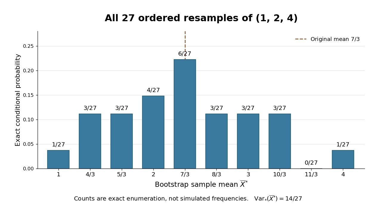

The conditional bootstrap variance of a sample mean gives a compact check on the enumeration. Each resampled draw has expected value and varianceAveraging three independent draws divides that variance by three:The exact conditional bootstrap standard error is . The original sample variance with denominator is , so its usual estimated standard error for the sample mean is . Their squared ratio is here; the difference follows from the empirical measure's denominator , not a numerical simulation error. Neither number is the known true sampling standard error of the unknown source probability distribution.
Configurational entropy Created 2026-10-18 Updated 2026-11-05
The part of entropy associated with the number of distinct spatial or occupancy arrangements consistent with chosen macroscopic constraints. For equally weighted configurations, the Boltzmann entropy formula gives the displayed expression. Unequal probabilities require over configurations. For indistinguishable empty sites among otherwise occupied sites, . Vibrational or internal degrees of freedom can contribute additional entropy even at fixed site arrangement.
Blume-Capel mean-field transition at zero single-ion anisotropy Created 2026-10-18 Updated 2026-11-05
For spins with ferromagnetic nearest-neighbour exchange and no single-ion anisotropy, a homogeneous mean-field approximation givesThe self-consistency equation is with . Its small- expansion is . Hence and, with , the nonzero branches satisfy . The critical exponent is the mean-field value , not an exact two-dimensional exponent. At zero source the finite-system equilibrium magnetization is zero by spin inversion symmetry; the broken branches describe the thermodynamic limit with a phase selected by a vanishing source.
Power-complement integral recurrence 2026-10-18
For and a nonnegative integer , integration by parts gives, when ,The endpoint term vanishes. ThereforeRepeated application yields . The integration by substitution also identifies with an Euler beta function. A related weighted integral follows immediately from the same substitution:
Trigonometric form of the beta function 2026-10-18
For positive real , substitute in the defining Euler beta function integral. The increasing substitution maps onto and has . Combining this factor with gives the displayed identity. Positivity of both parameters ensures convergence at the two endpoints, even when the integrand is unbounded there.
Equal-argument beta integral 2026-10-18
In , put . Then , and evenness givesThe further substitution turns this into . The symmetry of the Euler beta function yields the title identity. This proof works for every positive real , without requiring to be an integer or using the Gamma function.
In 2006, Zoran Hadzibabic, Peter Krüger, Marc Cheneau, Baptiste Battelier and Jean Dalibard split a cooled rubidium-87 cloud into two independent planar gases using an optical lattice. After release, the expanding sheets overlapped; absorption imaging recorded their matter-wave interference. Smooth fringe waviness revealed thermal phase fluctuations, while sharp dislocations indicated isolated vortices. The initial evaporative-cooling endpoint controlled the preparation; central fringe contrast served as a degeneracy proxy because direct thermometry in the lattice was difficult.[ref]
Berezinskii-Kosterlitz-Thouless Crossover in a Trapped Atomic Gas by Zoran Hadzibabic and others. Pages 1–2, preparation and readout; Fig. 1; temperature control and Fig. 2
Loss of extended coherence coincided with increased vortex signatures. The optical trap and finite cloud produced a crossover; tightly bound pairs were unresolved, and short-wavelength modes could contaminate high-temperature counts. These were observations of the vortex-unbinding mechanism, not a direct measurement of phase stiffness or a sharp homogeneous universal stiffness jump. The authors left the sample's superfluidity open.[ref]
Berezinskii-Kosterlitz-Thouless Crossover in a Trapped Atomic Gas by Zoran Hadzibabic and others. Pages 3–4, Figs. 3–4; geometry, invisible pairs, detection limits and final paragraph on unmeasured superfluidity
Single-vortex energy-entropy balance 2026-10-18
Consider an original counting example: a square two-dimensional XY model of side , a microscopic core radius , and a fixed phase stiffness . This deliberately neglects screening by other vortices. Away from a unit phase vortex, and . Integrating the Goldstone-mode effective free energy over an annulus givesBoundary shape changes finite terms. There are order core positions, so the positional entropy is , where is the Boltzmann constant. With , subtracting gives the displayed free energy.
For and , the dimensionless free energy cost is about at and at . The same logarithm appears in the cost and the positional reward: increasing the system size strengthens whichever has the larger coefficient. The corresponding one-defect Boltzmann factors, about and , are relative statistical weights, not normalized probabilities. The latter signals failure of a dilute single-defect estimate.
A single net phase vortex requires compatible boundaries: on a periodic sample use neutral pairs, as required by vortex charge neutrality. This argument identifies a possible threshold, but predicting the universal stiffness jump requires the renormalized phase stiffness, after smaller pairs have responded. It does not justify setting the transition temperature equal to a bare lattice coupling divided by a universal constant.
Neutral axis 2026-10-18
The neutral axis is the line in the cross-section of an elastic beam where longitudinal bending strain vanishes. For a homogeneous beam in pure bending, zero resultant longitudinal force gives , so the neutral axis passes through the centroid. Fibres on its opposite sides are stretched and compressed. The second moment of area about this axis controls the relation between bending moment and curvature.
All-to-one Bellman-Ford recurrence 2026-10-18
Keep the original all-to-one orientation of the Bellman inequalities: concerns routes from to a fixed sink , and belongs to the original directed edge . Initialize and for . The synchronous dynamic programming recurrence isIt prepends the first edge of a route instead of appending the last: is the minimum cost of a directed walk from to using at most edges. In particular, improving can improve labels on incoming directed edges . The same original directed edge therefore updates its tail in this convention, whereas single-source edge relaxation updates its head.
If no negative-cost directed cycle can reach , rounds suffice for every distance to , and automatically. This hypothesis concerns directed paths from the cycle to the sink, not paths from the sink to the cycle. In the base example with its original arrows and sink , the distances in order are . Once of weight is added, instead have distance to , while keeps distance and keeps .
More generally, precisely when can reach a negative-cost directed cycle that can reach . Thus the affected vertices are the ancestors of such a directed cycle. A negative-cost directed cycle unable to reach is irrelevant. Reversing all arrows makes a single source, turns these ancestors into descendants, and makes the detection and forward graph search above directly applicable. The right panel of the figure uses that reversal with sink ; its distances to equal the left panel's distances from .
Do not force the root to remain zero outside the hypothesis. Consider the two directed edges of cost and of cost , with sink . The recurrence gives and : the latter records one lap of a negative-cost directed cycle through . Repetition makes both unrestricted distances . Clamping at zero and omitting its update would instead leave the stationary labels , concealing that behaviour. Initialization specifies the cost of the empty directed walk; it does not forbid cheaper nonempty returns to the root. Cycle detection must test every relevant directed edge, including those whose relaxation updates the root.
Bellman-Ford negative-cycle detection 2026-10-18
A negative-cost directed cycle matters to a particular destination precisely when it is reachable from and can itself reach .[ref]
Lecture 17: Shortest Paths III: Bellman-Ford. 6.006 Introduction to Algorithms, Fall 2011 by Massachusetts Institute of Technology, 6.006 course staff; MIT 6.006, Lecture 17, p. 1: cycle between source and destination; p. 4: reachable-cycle corollary
Repeating it times adds times its negative total cost to a route. Thus the infimum of directed walk costs is , rather than the cost of a finite shortest directed walk. The distinction is about reachability, not simply the presence of a negative edge or a negative-cost directed cycle anywhere in the graph.Add of weight to the worked example. Now has total weight . Add also an isolated vertex with a self-loop of weight . From , the distances of are , because all four are reachable from the first negative-cost directed cycle. The source retains distance : no directed edge leads back to . The unreachable retains distance , despite its negative-cost self-loop.
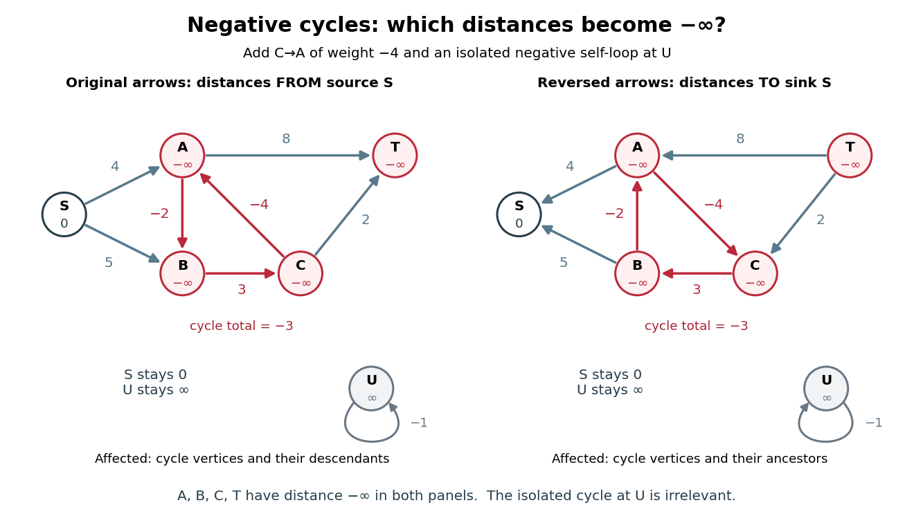
Relevant negative-cost directed cycles: descendants from a source become ancestors when every directed edge is reversed
. Details. 
For example, extra laps before proceeding to give costs . This construction also shows why requiring a directed path with no repeated vertices would change the problem: only directed walks permit arbitrarily many laps. Merely finding one reachable negative-cost directed cycle does not justify setting every reachable label to ; in the figure is a counterexample.
To detect and classify, perform full passes without clamping any label, then test all directed edges against a fixed copy of the resulting labels. Collect heads of edges satisfying and . An empty collection certifies that no negative-cost directed cycle is reachable from . Otherwise run graph search forwards from all collected vertices: precisely the reached vertices have distance . A vertex unreachable from still has distance ; each remaining vertex has its finite shortest distance.
Why is this classification exact? Every unaffected reachable vertex already has its shortest distance after passes, since any route ending there avoids reachable negative-cost directed cycles. Thus it cannot be the head of a strict improvement, or be reached from such a head. Conversely, all vertices on a reachable negative-cost directed cycle have finite labels by that time. If none of its edges could improve a label, summing around it would imply . At least one of its heads is therefore collected, and the forward graph search reaches the entire directed cycle and every affected descendant. Detecting a directed cycle alone and marking its descendants are separate tasks; finite intermediate labels in the affected region are not answers.
Synchronous Bellman-Ford recurrence 2026-10-18
For the single-source problem, let be the minimum cost of a directed walk from to using at most edges. Set and for , use for finite , and let a minimum over an empty set be . ThenEvery entry on the right comes from the previous round, requiring separate old and new arrays. The proof is the last-edge decomposition: a permitted directed walk either already uses at most edges, or ends with some after a prefix using at most . Conversely, each candidate describes a permitted directed walk. This dynamic programming viewpoint gives an exact meaning to every intermediate label, even when negative-cost directed cycles exist. Apply the formula to the source too: its initial zero is not a permanent constraint.
If no negative-cost directed cycle is reachable from , removing repeated-vertex portions of a directed walk cannot increase its cost. Whenever a destination is reachable, some shortest directed path therefore uses at most edges, and . Unreachable vertices keep distance . For in-place passes, every finite label still comes from a discovered directed walk; moreover, pass has offered every prefix of length of a shortest directed path, regardless of scan order. Its labels can improve faster than the synchronous labels, while the same upper bound on passes remains valid. This is why repeated local corrections eventually settle a global shortest path problem.
Locality loophole 2026-10-18
The locality loophole permits a station's outcome to be influenced by the distant setting through an ordinary signal arriving before readout. Spacelike separation excludes such communication at or below the speed of light. Fast changes only help if the relevant choice and detection events have the required timing. Predictable switching also leaves open correlations with earlier settings; closing a communication channel does not prove measurement independence.
Detection loophole 2026-10-18
The detection loophole arises when missed events allow the retained sample to depend on settings and hidden variables. For example, a local hidden-variable theory may retain different underlying pairs at different polarizer angles. Applying the CHSH inequality to that selected sample does not test the original setting-independent ensemble. A valid protocol specifies outcomes and trials, including failures, or justifies an appropriate fair sampling assumption. Subtracting accidental coincidences addresses background contamination; it does not by itself repair this selection problem.
In 2015, Marissa Giustina, Anton Zeilinger and collaborators combined spontaneous parametric down-conversion with rapid random analyzer choices and efficient transition-edge sensors. Local records included settings and detector signals; their Bell inequality used detected and undetected trials, avoiding fair sampling. Locally fixed time slots prevented coincidence-based trial selection. Calibrated optical and electrical delays checked spacelike separation of each choice from the remote readout. The violation addressed detection and locality together. Measurement independence still requires assumptions about the hidden state's origin; the experiment cannot exclude every possible common cause of source and settings.[ref]
Photonic entanglement-swapping experiment 2026-10-18
In 1998, Jian-Wei Pan, Dik Bouwmeester, Harald Weinfurter and Anton Zeilinger created two photon pairs by two passages of a pulsed pump through a crystal using spontaneous parametric down-conversion. Interfering the inner photons at a nonpolarizing beam splitter implemented a partial Bell-basis measurement. Narrow optical filters and spatial filtering removed distinguishing information; changing the outer polarizer bases checked the conditional correlations. Fourfold detections selected the entanglement swapping events. The reported interference supported conditional quantum entanglement, but the paper reserved a statistically significant Bell inequality violation for improved visibility; it was not a demonstration closing the detection loophole.[ref]
Experimental Entanglement Swapping: Entangling Photons That Never Interacted by Jian-Wei Pan and others. pp. 3892-3894, Eq. (3), Figs. 2-3; visibility discussion
The ideal calculation makes the distinction between conditional and unconditional quantum states explicit. Start with spin singlet states , where and denote orthogonal photon polarizations. Taking the inner product with gives : expanding the four terms leaves precisely the two antisymmetric outer terms. That Bell-basis measurement outcome has probability and leaves the outer pair in a spin singlet state. Ignoring the inner outcome instead leaves the outer density matrix , a maximally mixed state. A conditional preparation flag is useful for later Bell tests only with the timing and setting conditions in setting-independent heralding preserves Bell locality.
Aspect switching experiment 2026-10-18
In 1982, Alain Aspect, Jean Dalibard and Gérard Roger used a calcium cascade and an acoustic standing wave in water to route each photon toward one of two fixed polarizers. Switching took about , against for light to cross between stations. Photomultiplier coincidence circuit rates, with delayed-background subtraction and polarizer-removal normalization, violated their Bell inequality. Supplementary polarizers checked each channel against Malus's law. The timing attacked the locality loophole, but the authors emphasized that switching was quasiperiodic, not random; incomplete switching and inefficient collection also limited the test. Its normalized statistic differs from the CHSH inequality convention used below.[ref]
Experimental Test of Bell's Inequalities Using Time-Varying Analyzers by Alain Aspect and others. pp. 1805-1807, Figs. 2-4; final discussion
There are unlisted articles, also show them or only show them.