
One-Mile Telescope 2026-10-18
The One-Mile Telescope used three steerable 60-foot dishes: two fixed, one rail-mounted. The movable–fixed pairs supplied two baselines simultaneously. Twelve-hour tracks at successive rail positions sampled projected spacings. Phase-switching receivers measured in-phase and quadrature correlations; adjustable delay and phase rotation compensated tracking.[ref]
The Operation of the Cambridge One-Mile Diameter Radio Telescope by Bruce Elsmore and others. Elsmore et al. (1966), sections 1–2, pp. 87–92, Figures 1–2
The readout was correlation versus time. Reference-phase subtraction should leave constant point-source phase; position offsets produce predictable variation. A source near the field's declination supplies a collimation check. Structure, instrumental error and sampling artefacts need separating.[ref]
The Operation of the Cambridge One-Mile Diameter Radio Telescope by Bruce Elsmore and others. Elsmore et al. (1966), section 4(a), p. 93; Appendix, p. 95
Radio interferometry Created 2026-10-18 Updated 2026-10-20
Radio interferometry measures the spatial coherence of received radio waves. At two antennas, a receiver preserves the relative wave phase, compensates the geometric delay for a chosen phase centre, and averages a product of one signal with the complex conjugate of the other. In a complex-signal description this correlation is . Its real and imaginary parts carry two complementary components of the complex visibility; measuring only the received powers discards the relative wave phase needed for general imaging.
A finite frequency band makes delay compensation essential. If the residual delay is , the residual wave phase varies by across a band of width . Averaging these differently oriented complex contributions reduces the correlation. For an ideal rectangular band the multiplicative factor is . A phase correction at just the central frequency cannot remove this variation across the band. Long time averages can likewise smear a changing signal.
Semiconductor transport evidence for localization Created 2026-10-18 Updated 2026-10-20
Nevill Francis Mott's 1977 lecture discusses silicon deposited in a glow discharge. Injected electrons provided a drift-mobility readout; electrical conductivity and temperature dependence tested localized-state transport and excitation toward a mobility edge. Varying temperature distinguishes transport regimes. The lecture gives no contact geometry or timing circuit here, so none is inferred. Its Figure 2 is schematic, not measured data.[ref]
Electrons in Glass by Nevill Francis Mott. Electrons in Glass, pp.404–406, Fig.2 and discussion of glow-discharge-deposited silicon; inspected institutional mirror www.nevis.columbia.edu/~haas/documents/physics_nobel_lectures/physics71-80-2.pdf
This evidence motivates a transport question beyond the closed-chain eigenvalue problem: how does a prepared charge disturbance move under the conditions of a real sample? The numerical figures above supply neither drift-mobility measurements nor a model of the deposition process. Finite-size concentration alone cannot reproduce an experimental electrical conductivity curve.
Finite temperature permits phonon-assisted hopping between localized eigenstates or thermal excitation toward a mobility edge; localized states therefore need not imply zero measured electrical conductivity at every nonzero temperature.[ref]
Electrons in Glass by Nevill Francis Mott. Electrons in Glass, pp.405,407, localized-state hopping and thermal excitation
Real dephasing destroys the relative wave phases needed for long-path interference. Observing coherent confinement requires the distance over which those wave phases survive to be long enough to explore the localized region, and the sample to be large enough to resolve it. Temperature alone is not an automatic switch: the actual inelastic processes set the relevant scales. Static elastic wave scattering preserves coherence within each realization. Loss of the ensemble-averaged coherent field through random wave phases is therefore not, by itself, physical dephasing of an individual sample.
One-dimensional Anderson chain Created 2026-10-18 Updated 2026-10-20
Consider a noninteracting electron in a finite tight-binding model with open ends:The vectors form an orthonormal basis of site states. The hopping energy is ; it is not the time coordinate. Draw each independently from the continuous uniform distribution on and then hold it fixed. The disorder strength is dimensionless. Open ends mean no hopping bond connects sites and ; equivalently set . There are no electron interactions, phonons or wave absorption in this model.
The eigenvalue equation in the interior isAs a simple local calculation, if a state's peak is at , a neighbouring site with receives a small leading contribution . Several successive large mismatches multiply small factors. This explains why large disorder can restrict spreading, but is not a proof of Anderson localization: near-resonant denominators and alternative interference paths prevent treating this expansion as uniformly valid.
For the first original calculation, take , , and the fixed random seed . Diagonalizing the resulting real symmetric matrix with
numpy.linalg.eigh and selecting the eigenvalue closest to zero gives , a probability peak at site , and . The selected eigenvector has total probability one. This is one chosen realization, not a disorder average or a measured specimen.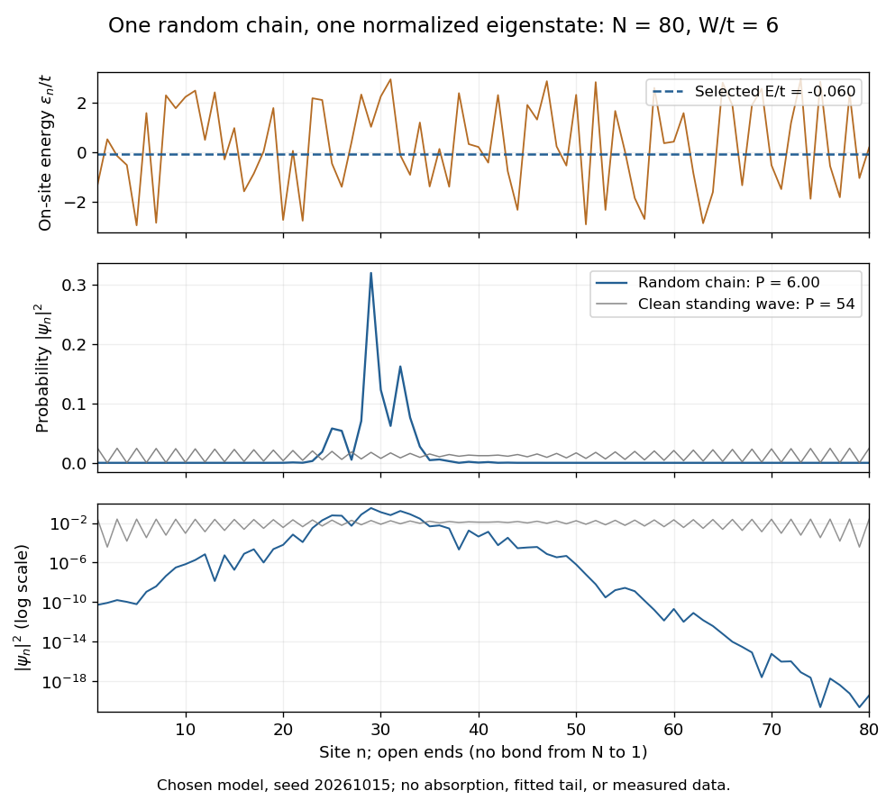

The clean comparison needs care. With , the open chain has standing wavesFor even , the identity and finite trigonometric sums give , hence . Thus the clean -site comparison has , although it extends across the chain. Extended does not mean uniform probability. For odd , the special central mode has zeros on alternating sites and instead ; the even-size assumption avoids that exception.
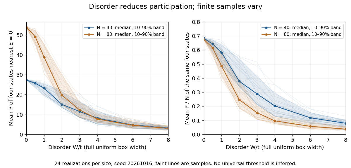
The second original calculation compares and over . For each size, draw independent site patterns using seed , with the size included in the random-seed construction. Scale each fixed pattern across disorder strengths. At every point, average over the four energy eigenstates closest to . The solid line is the median across these sample averages; shading spans their th–th percentiles. The selected states can change as varies: lines connect one sample's selections rather than tracking a single mode.
Participation ratio varies across disorder realizations and finite chain sizes
. Original One-dimensional Anderson chain calculations. Faint lines show individual sample averages, solid lines their medians and bands their th–th percentiles. The left panel plots ; the right divides by site count . These finite samples illustrate concentration and variability, without a fitted critical disorder. Details.
At the two clean values are and . At , the computed median sample averages are approximately and . In the latter regime, doubling hardly changes the typical occupied site count, so falls. At weak disorder the larger chain permits more spatial extent. Neither a single curve nor the overlap of finite-size bands proves the infinite-system statement under mobility edge; a long localization length can hide confinement in either size.
Mobility edge Created 2026-10-18 Updated 2026-10-20
A mobility edge separates localized from extended energy eigenstates on the energy axis. Three-dimensional disordered models can have both. In the infinite one-dimensional tight-binding model with independent continuous random site energies, all states are localized for any nonzero disorder, with probability one. This statement excludes specially correlated disorder.[ref]
Local Moments and Localized States by Philip Warren Anderson. Local Moments and Localized States, pp.395–396, mobility edge and one-dimensional localization; institutional mirror as above
A mobility edge is not a band gap: states can exist on both sides of , but differ in spatial extent. For electrons, the location of the Fermi energy relative to a mobility edge matters for low-temperature electrical conductivity. A three-dimensional sample need not have an extended interval at every disorder strength. In particular, the finite one-dimensional calculations below neither locate a three-dimensional mobility edge nor establish a nonzero universal critical disorder.
Localized eigenstate 2026-10-18
A localized eigenstate is an energy eigenstate whose spatial weight remains concentrated near some position as the system grows. An exponentially localized eigenstate has a decaying envelope characterized by a localization length. A small participation ratio measures concentration in a chosen site basis; it does not by itself establish an exponential tail or a transport law.
An energy eigenstate changes only by an overall wave phase under time evolution, whether localized or extended. Its stationary probability distribution alone therefore does not distinguish transport mechanisms. The important distinction concerns spatial extent and how superpositions of energy eigenstates carry or retain a disturbance. A wave packet assembled from localized eigenstates with nearby centres can remain confined, whereas extended modes can support propagation.
Mobility gap Created 2026-10-18 Updated 2026-10-20
An energy interval with no extended bulk energy eigenstates available for transport. It can contain localized eigenstates and have a nonzero density of states; a mobility gap need not be a spectral gap.
Accounting method 2026-10-18
The accounting method charges operations enough to pay for their work and save credits for later work. A nonnegative balance from an initially empty account makes every prefix's total charge an upper bound on its actual cost. Choosing the balance to be gives the potential method; the ledger for dynamic array doubling illustrates this equivalence.[ref]
https://www.math.u-szeged.hu/~hajnal/courses/MSc_AlgoBony/2021/Tarjan.pdf. Robert Endre Tarjan, Amortized Computational Complexity, section 2, pp. 307–308: banker's credits and equivalence with the potential viewpoint
// Destination: computer-science.bigb
Aggregate analysis 2026-10-18
Aggregate analysis bounds the total cost of a whole sequence directly, then divides by its length to obtain an amortized bound. Summing the copied capacities as a geometric series in dynamic array doubling is an example.
Potential method 2026-10-18
The potential method assigns a number to each state of a data structure. Let be the state after operation , , and its actual cost. Its amortized cost is the actual cost plus the change in potential. Summing and cancelling adjacent potentials gives a telescoping sum:If and every reachable , the sum of amortized costs bounds the actual total for every prefix. A nonzero initial potential contributes the explicit additive term . Potential is proof bookkeeping; the algorithm need not store it.[ref]
Lecture 20: Hash tables and amortized analysis. CS 312 at Cornell University; CS 312, lecture 20, “Amortized analysis”: definition of amortized time and cancellation of successive potential changes
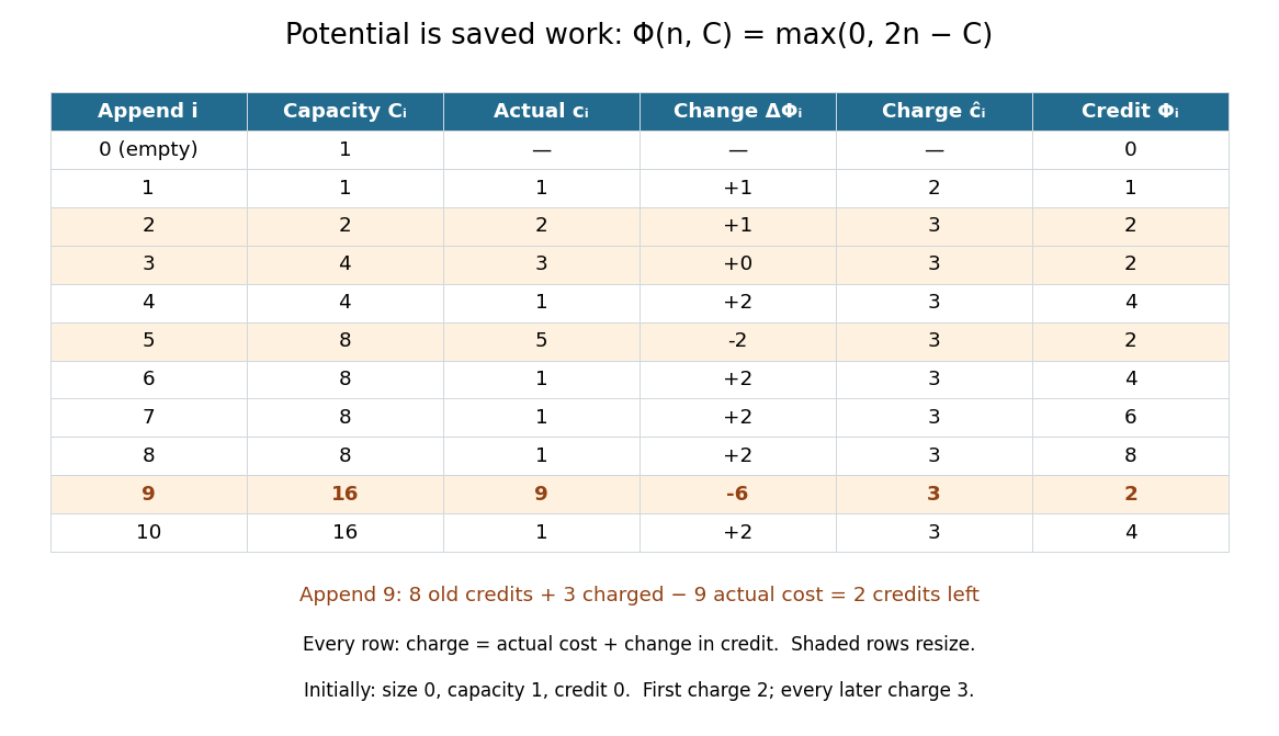
For dynamic array doubling, chooseThe potential method now starts at . After every nonempty reachable state, , so the maximum equals . There are just three cases for append:
For every , the total charge is , and the telescoping sum provesThis agrees exactly with . The unmodified choice has initial value , so calling it nonnegative at the empty state would be incorrect. It also works if that initial constant is retained in the identity; alternatively, starts at zero and is nonnegative on these reachable states. The maximum above keeps a literal nonnegative credit balance from the beginning. The proof covers append alone; allowing reserve or arbitrary deletion changes the reachable states and requires a new argument.

Dynamic array doubling Created 2026-10-18 Updated 2026-10-31
Consider a dynamic array holding fixed-size entries. Its size is the number of occupied slots and its capacity is the number of allocated slots. Start with , . The only operation is append: if , allocate a new array of capacity , copy the existing entries, and release the old array; then write the new entry and increase by one. There is no reserve operation, deletion or shrinking in this model.
Count one unit for writing the new entry and one unit per existing entry copied during resizing. Thus the th append has actual cost without resizing and when the old capacity is full. Copying an entry, including its read and write, is one counted action. Allocation, deallocation, index arithmetic operations and the initial one-slot allocation are outside this exact count. If these add only a constant per ordinary append and a linear cost per resize, the Big O notation conclusions still hold, with different constants; costly entry copies require their own cost model.
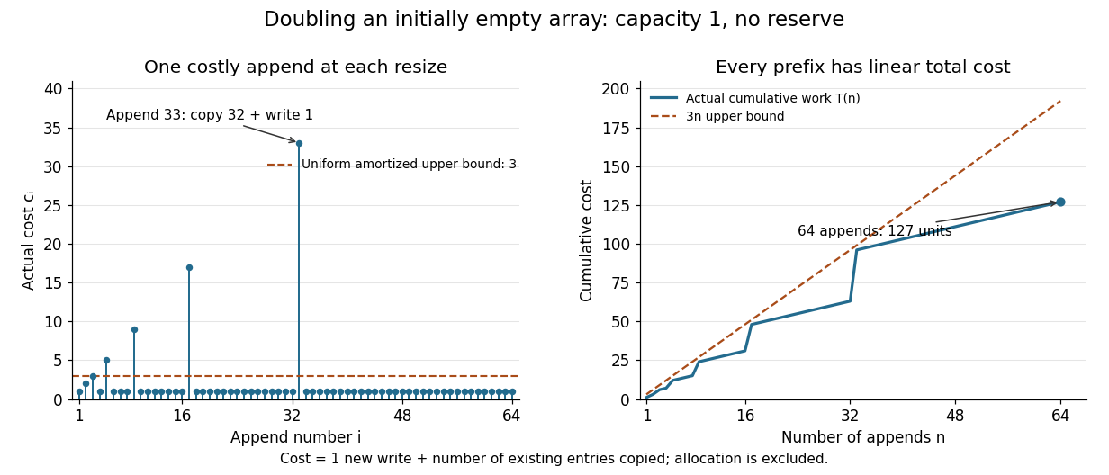
The first ten costs are . For example, append copies eight entries and writes one, so . At that point the capacity becomes , but the total cost of all nine appends is only .
For , the final capacity is . Every earlier capacity was copied once. This geometric series sums to , including the empty sum when . Therefore aggregate analysis gives the exact totalConsequently , so append has amortized cost in Big O notation for every prefix from this empty initial state. The values being appended do not affect the count. In contrast, an append to a full dynamic array with entries costs : its worst-case cost is , and actually grows linearly along full-capacity states. A bound on total work does not promise a constant response time for each call.
Individual append costs and cumulative work under dynamic array doubling
. The spikes include every copied entry and the new write. At append 33 the actual cost is 33; at append 64 the total cost is 127. Every prefix lies below the line . Details.
The same policy controls computer memory: after each completed append, for , so fewer than slots are unused. This is a bound on the retained backing array, with fixed-size slots. During a resize from full capacity to , a copying implementation can temporarily hold both arrays, totalling allocated slots before releasing the old one. Thus the retained-capacity bound does not bound this temporary peak by twice the live size. Allocator metadata and separately allocated objects are additional computer memory costs.
The geometric series is the source of the efficiency. If capacity instead increases by one each time, the same count becomes , a quadratic total. Dynamic array doubling buys a linear total with bounded spare capacity, even when the final length is unknown.
Why add the daughter four-momenta? Consider a selected combination of final particles withUsing the Minkowski metric, its scalar square isIn the combination's center-of-momentum frame, its total momentum vanishes and its total energy is . Therefore , givingLorentz transformations preserve this scalar square, so the reconstructed invariant mass does not depend on the combination's laboratory motion. It includes relative kinetic energy and need not equal the sum of the daughter rest masses. A random pair has an invariant mass too; that number does not itself establish a common parent.
For two daughters, expanding the square and substituting each energy–momentum relation givesHere and are masses, not energies. Reporting in and momenta in is equivalent to calculating numerically with and in . Setting in natural units suppresses these conversion factors; it does not change the measured quantity.
Alvarez's lecture illustrates invariant mass searches with combinations and contrasts resonance lifetimes near with the much longer lived states the chambers originally targeted. These resonances decayed before producing a resolvable parent track.[ref]
Recent Developments in Particle Physics by Luis Walter Alvarez. UCRL-18696, printed pp. 46–47, Figs. 15–17: effective-mass histograms and short lifetimes
Operationally, choose a reaction hypothesis, require an acceptable bubble-chamber kinematic fitting result, and form specified daughter combinations. Accumulate their invariant masses in a histogram across events. A particle resonance is inferred from the ensemble's dynamics; its short-lived parent is not directly photographed. Daughter tracks can be visible even when the production and decay positions of the parent cannot be separated. Wrong combinations create background, and several combinations from one event are statistically correlated.
Bubble-chamber kinematic fitting 2026-10-18
Alvarez describes a progression from measured coordinates to momenta and angles, then conservation-constrained fits testing alternative track identities. Computer programs made the repeated tests practical; an insufficiently constrained event could retain several hypotheses.[ref]
Recent Developments in Particle Physics by Luis Walter Alvarez. UCRL-18696, printed pp. 30–33: HYDRO, PANG, GUTS, KICK and SUMX
A mathematical formulation explains what such a fit can establish. Let collect measured momenta and angles, with positive-definite covariance matrix . For a chosen reaction hypothesis, adjust them to by minimizing a generalized least squares objective,The constraints express four-momentum conservation and any independently known daughter masses. For each proposed identity, calculate energy from the energy–momentum relation, . A missing neutral particle adds unknowns; a measured decay vertex can add geometric constraints. Compatibility depends on the measurement errors and the independent constraints, not just the smallest raw among unrelated fits.
A simple independent check uses a single momentum conservation constraint. Suppose two measured one-dimensional momenta are and , each with independent standard deviation , and a stipulated parent at rest requires their sum to vanish. Minimizing the two equal-weight squared changes gives fitted values and , with . A fit repairs a mismatch according to a hypothesis; it does not prove that hypothesis. This one-component illustration is not a complete reaction fit.
Bubble-chamber stereo reconstruction 2026-10-18
Stereoscopy supplies depth because different cameras see different projections of the same track. A functional reconstruction first matches the same interaction vertex and track segments across views. A calibrated lens and window model maps each measured image coordinate back to a ray inside the liquid. Refraction at the windows must be included. Intersecting the rays, or finding their closest agreement when measurements have errors, estimates three-dimensional coordinates. Several points then determine a trajectory, rather than only a projected arc.
An original ideal-camera model makes the geometry explicit. Take two parallel pinhole cameras with centers and , focal length , and optical axes along . Use virtual image planes in front of the pinholes so that image coordinates have the same orientation as the scene. A point then givesSubtracting the horizontal image coordinates gives disparity , henceFor stipulated , , , and , the reconstructed point is . These are ideal optical inputs, not dimensions of Alvarez's apparatus. This model omits refraction and lens distortion; actual calibration replaces its simple ray geometry. Since , the same disparity error gives worse depth precision for distant points.
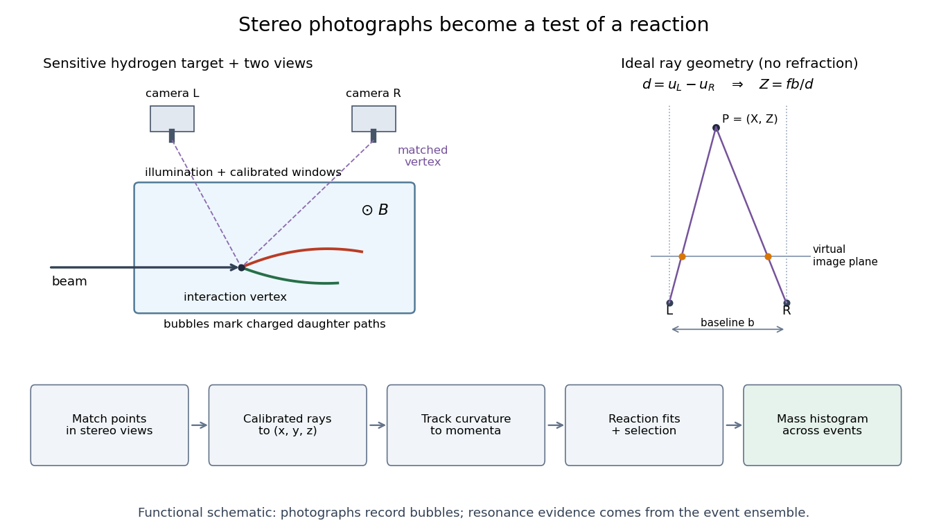
From stereo bubble photographs to coordinates, momenta and an event ensemble
. Original functional diagram. The chamber, camera positions and tracks are schematic, not a historical mechanical drawing. The parallel-camera ray construction illustrates an idealized model without refraction. Details.
The Lorentz force then supplies a momentum scale. With magnetic field uniform and negligible stopping power over a fitted segment, bubble-chamber track readout gives . The local three-dimensional helix tangent supplies the missing direction: if is its angle to the field, . In practical units,Here is the elementary charge and the speed of light. A short, almost straight arc poorly constrains its radius of curvature; a visually sharp track can therefore have poor momentum precision.
Superallowed beta decay Created 2026-10-18 Updated 2026-10-20
An especially strong allowed beta decay, conventionally including pure Fermi transitions between isobaric analog states. Those states have closely related spatial and spin structure, so the isospin ladder operator has a large overlap. A assignment alone fixes the allowed Fermi character, but does not establish analog-state overlap or a large rate; a small comparative half-life supplies additional evidence.
Anti-aliasing filter Created 2026-10-18 Updated 2026-10-25
An anti-aliasing filter suppresses signal components outside the intended acquisition band before sampling. For voltage recording it is an analogue filter ahead of the analog-to-digital converter, with a transition band allowed below half the sampling rate. Once two frequencies have become indistinguishable through aliasing, a digital filter generally cannot recover the lost distinction. The Nyquist–Shannon sampling theorem concerns an already bandlimited function; a physical filter approximates that prerequisite.
Drift-diffusion decay time Created 2026-10-18 Updated 2026-10-31
For constant diffusion coefficient and drift velocity , the balance gives the characteristic length and time . The fundamental Gaussian distribution of the advection-diffusion equation has a fixed-position exponential factor . Total probability is still conserved: this describes probability moving away from a fixed observation region, rather than disappearance of the particle. At zero drift, this finite exponential time scale is absent.
Adiabat Created 2026-10-18 Updated 2026-10-25
An adiabat is a curve representing a quasistatic adiabatic change. In a reversible description it is also a curve of constant entropy. For an ideal gas with constant heat-capacity ratio , it obeys . A general irreversible adiabatic process need not follow this equilibrium-state curve and can produce entropy.
Limits of adiabatic demagnetization 2026-10-18
Three distinct effects spoil indefinite cooling: extra entropy outside the spin subsystem, additional magnetic energy scales, and irreversible heat or work input. They can be distinguished with a thermodynamic derivative. For a smooth equilibrium Helmholtz free energy obeying , a Maxwell relation givesHere is the total heat capacity participating in the stage's thermal equilibrium. The ideal model has . If its spins share temperature with a field-independent lattice and load of combined heat capacity , thenThe positive slope still means cooling when , but its smaller magnitude gives less cooling per fractional field reduction. For example, a low-temperature Debye model gives a lattice entropy proportional to . As that lattice entropy falls, the spins take up the released entropy; can no longer remain constant. A weak enough coupling to neglect its equilibrium interaction energy can still be strong enough to exchange heat on the sweep timescale.
Interactions between magnetic moments, including exchange interaction and the fields of neighboring magnetic dipole moments, introduce energy scales that do not vanish with the applied . Once they compete with or , the independent-site partition function fails. Correlations and possible magnetic ordering alter the available magnetic entropy and the cooling curve. Simply setting the external magnetic field to zero does not eliminate those interactions. Different refrigerants therefore need their own measured equilibrium properties; there is no universal final temperature from the applied-field ratio alone.
Finally, a real open heat switch has residual thermal conductance; supports, wires and radiation carry incoming heat. Field changes may also dissipate energy. Locally near thermal equilibrium, with incoming heat rate and internal entropy production rate , the stage balance becomesThis uses a common stage temperature; a non-equilibrated load requires separate balances. The sweep must allow spin-lattice relaxation while remaining fast enough to limit accumulated parasitic heat. At fixed , the same balance explains warming and finite hold time. Useful refrigeration is the controlled absorption of a load's heat during that finite interval, followed by a renewed isothermal process of magnetization to export its entropy.
William Francis Giauque's 1949 lecture, Some Consequences of Low Temperature Research in Chemical Thermodynamics, credits Peter Debye with an independent proposal. It describes gadolinium sulfate octahydrate in a jacket immersed in liquid helium, with an external solenoid. Exchange gas conducts away heat during magnetization; evacuation isolates the sample before field reduction. A liquid-nitrogen shield reduces radiative heat transfer. Its photograph identifies the 1933 apparatus operated with Duncan Peck MacDougall. An inductance bridge reads the sample's magnetic susceptibility; measuring coils remain outside the evacuated jacket in liquid helium. Increasing magnetic susceptibility indicates cooling, but converting it to temperature using Curie's law becomes approximate as that law fails.[ref]
Some Consequences of Low Temperature Research in Chemical Thermodynamics by William Francis Giauque. Giauque, Nobel lecture, pp. 237–245, Figs. 16–20 and 23–25
The measurement logic deserves a separate check. A changed inductance alone is not an absolute temperature calibration: the sample geometry, applied measuring magnetic field, and constitutive response enter the inference. A modern control would compare the susceptibility-based thermometer with an independently calibrated thermometer over their common range, check recovery after repeated sweeps, and measure subsequent warming to bound incoming heat. These are proposed controls derived from the readout principle, rather than additional procedures attributed to the 1933 experiment. The historical working salt has a richer magnetic level structure than the illustrative two-level paramagnetic cooling model.
There are unlisted articles, also show them or only show them.