
Magnetic entropy Created 2026-10-18 Updated 2026-10-20
Magnetic entropy counts the uncertainty in the occupied magnetic microstates. For independent localized magnetic moments with one-site probabilities ,where counts sites and is the Boltzmann constant. This is the Gibbs entropy for the magnetic degrees of freedom. Equal occupation of two states gives ; certain occupation of one state gives zero. Calling this disorder is useful only if the relevant states and their probabilities are specified. In an interacting material, correlations generally prevent replacing the many-body Gibbs entropy by this sum of independent one-site contributions.
Increasing the magnetic field at fixed positive temperature favors lower magnetic energy levels, reducing magnetic entropy. During ideal isolated demagnetization, both the level separation and temperature fall together, leaving the occupation probabilities unchanged. Thus the independent-spin idealization cools without increasing spin disorder along the isolated leg. When a real crystal's vibrating lattice also cools, its lost entropy can instead be taken up by the magnetic degrees of freedom. The conserved quantity is the total entropy of the thermally isolated stage, including any attached load in thermal equilibrium.
Discontinuous additive function 2026-10-18
Assuming the axiom of choice, Cauchy's functional equation has solutions that are not linear maps over the real numbers. Regard as a vector space over the rational numbers. Because is an irrational number, and are linearly independent over . Zorn's lemma extends them to a Hamel basis ; assigning arbitrary real outputs to its basis vectors and extending by finite rational linear combinations gives an additive function.[ref]
Zorn’s Lemma and Some Applications by Keith Conrad. §4, printed pp. 19–20, Corollaries 4.2 and 4.5: basis extension and an additive map not of the form cx
For a particular choice, assign and for every . Every real number has a unique finite linear combination with finite and . Definewhere the coefficient is zero if . The uniqueness of the Hamel basis representation makes this definition unambiguous, and adding the coefficients proves . On the rational two-dimensional vector subspace spanned by and , the rule is particularly simple:For instance, and give , , and . Thus the map still preserves addition, even though rules out being a linear map over the real numbers.
The rational approximants from additive function continuous at one point is linear expose the failure of continuity: but . Moreover while . The map is continuous nowhere, since continuity at any point would imply additive function continuous at one point is linear. It is unbounded on every interval of positive length by additive function bounded on an interval is linear.
The axiom of choice is used to obtain the Hamel basis; the coefficient rule does not provide an explicit way to find the representation of an arbitrary real number. A plot sampled only at rational numbers would show exactly the same values as , so that plot cannot reveal this discontinuous additive function.
Let be an additive function. Suppose for all in a nondegenerate interval , meaning . Then is continuous everywhere and . A finite bound on even one such interval is enough; a bound at one isolated point is not.
Here is a proof outline that turns a finite bound into arbitrarily small outputs. Set and . If , then both and lie in , so Cauchy's functional equation givesGiven , choose a positive integer with . For , the argument lies in , and rational homogeneity of an additive function givesThis proves continuity at zero. Now additive function continuous at one point is linear completes the proof. The key mechanism is that repeated addition magnifies a tiny input without escaping the bounded region, forcing the original output to be small.
Rational homogeneity of an additive function 2026-10-18
For every additive function , every real number , and every rational number , one has . This is the scalar multiplication part of being a linear map over the rational numbers.
First gives , and gives . Repeated addition gives for each positive integer , and the negative case follows from the sign identity. If with and , thenNo continuity was used. In particular fixes , , and every other rational value, even for a discontinuous additive function.
Blazar Created 2026-10-18 Updated 2026-11-05
A blazar is an active galactic nucleus whose relativistic jet is viewed close to its direction of motion. Relativistic beaming enhances the apparent radiation from approaching material and changes observed variability timescales. Its extreme brightness is therefore affected by orientation as well as by the power supplied by black-hole accretion.
A source's brightness and spectrum do not directly identify the particles responsible for every emission component. Radio through gamma-ray observations and their timing help distinguish candidate mechanisms, while TXS 0506+056 illustrates the additional information supplied by a possible association with high-energy neutrinos.
Inverse Ackermann function 2026-10-18
For the displayed Ackermann function convention, one possible inverse-growth scale is for positive integers . It gives through , from through , and from through . Several inverse Ackermann function conventions occur in algorithm analysis; changing convention can shift these small values without changing the very slow growth relevant to the disjoint-set data structure. This inverse-growth definition does not invert a two-variable function as an ordinary one-variable inverse function.
Titrant 2026-10-18
A titrant is the reagent added in measured quantities during a titration; its known concentration and delivered volume determine the added amount of substance.
Titrant standardization 2026-10-18
Titrant standardization determines the actual titrant concentration by reaction with a known inventory, often a primary standard. It is distinct from calibrating the delivered volume or a glass electrode's response. For a known monoprotic acid inventory and a suitable blank-corrected endpoint,An original illustrative standard of requiring , with matched blank , gives . The measured quantities here are stipulated examples. Independent solution preparation and volumetric calibration tests the pipette, burette, and volumetric flask; titrant standardization tests the reacting inventory per delivered volume.
The useful chain is known mass, known composition, known amount of substance, and then a measured titre through a specified stoichiometry. If each standard unit consumes units of titrant, the general inventory equation is , where is the corrected titre. The one-to-one formula above has . A titration endpoint supplies an observable stopping rule; whether it represents the equivalence point accurately remains a separate question. Standardization endpoint and blank bias makes the direction of the resulting error explicit.
Acid-base titration measurement 2026-10-18
The institutional experiment The Potentiometric Titration of an Acid Mixture, from Massachusetts Institute of Technology's 5.310 Laboratory Chemistry, determines hydrochloric acid and phosphoric acid inventories. Dried potassium hydrogen phthalate standardizes sodium hydroxide. A volumetric pipette selects an acid aliquot, diluted with water in a beaker. A burette feeds a stirred sample beside a glass electrode; the apparatus isolates the sample from stirrer warming. The burette is conditioned with titrant and its tip freed of bubbles. Stable pH and added volume are recorded, with smaller additions near the transition. Controls include replicate standardizations, a consistent pale-pink phenolphthalein endpoint, and a standard buffer solution check between sample runs. The readout supports inventory estimates through known stoichiometry; it does not directly count molecules.[ref]
The same protocol requires drainage time for burette readings and warns that an undelivered hanging drop spoils the association between volume and pH. Its color-persistence wording differs between the main paragraph and footnote, so a reproducible titration endpoint needs an explicitly chosen criterion. Its acid mixture is not the single-strong acid ideal model above.[ref]
The Potentiometric Titration of an Acid Mixture (MIT 5.310 laboratory handout). Printed Titration-6, main endpoint paragraph and footnote 6; Titration-8, hanging-drop warning
A distinct control appears in Process Measurement Procedures: Sulfuric Acid Emissions, §1.4.4.2: the phenolphthalein standardization is repeated with water replacing the acid, matching the sample aliquot and indicator quantity. The volume needed for the same pink endpoint is subtracted from the sample reading.[ref]
Process Measurement Procedures: Sulfuric Acid Emissions by R. Maddalone and N. Garner. Process Measurement Procedures: Sulfuric Acid Emissions, printed pp. 26–27, §1.4.4.2, indicator-blank paragraph, NOTE, and procedure steps 1–3
The independent bookkeeping for such a matched blank is , assuming one-to-one neutralization and equal background consumption. A blank cannot correct an unmatched chemical reaction or guarantee exact coincidence of endpoint and equivalence point. Subtracting pH readings would not give this inventory correction, because pH is a logarithm. Repeatability constrains scatter; an independently known check sample also tests systematic bias. Carbon dioxide uptake, incomplete mixing, electrode drift, and uncertain titrant concentration limit the inference.
Strong acid titration model 2026-10-18
Consider an original ideal model: of hydrochloric acid at , titrated with sodium hydroxide at . Treat these numbers as exact model inputs. Assume complete dissociation of an ionic compound, complete strong acid ionization, additive volumes, uniform mixing, and activity coefficients equal to one. Use stipulated , approximately appropriate near . These are calculated pH values, not measurements of these materials.
The chemical equation for neutralization isInitial acid inventory is , so the equivalence point is . Added water does not change this inventory. But the final volume , including the titrant, determines all concentrations.
Keep self-ionization of water even at the equivalence point. With , define the dimensionless acid excess , hydronium level , and hydroxide level byThe sodium cation and chloride anion inventories fix the electric charge balance , while chemical equilibrium gives . Eliminating yields a quadratic equation with exactly one positive root. For stable calculation on either side, writeThe second expression follows by multiplying by ; it avoids subtracting two nearly equal large quantities on the alkaline side. A logarithm acts on the dimensionless , as required by the pH definition.
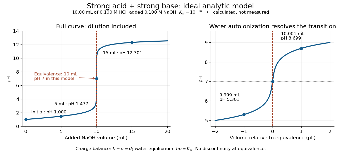
An ideal strong acid titration curve stays smooth through its equivalence point because of self-ionization of water
. Original analytic model for of hydrochloric acid and sodium hydroxide, with . Both panels use the complete electric charge balance and ideal chemical equilibrium. The right panel resolves microlitre additions around the equivalence point. The marked points are calculated, not measured. Details.
At , the excess is in , giving and pH . At , excess hydroxide is in , giving and pH . Neglecting dilution would give the wrong values even far from the equivalence point.
Exactly at , and , giving pH in this model. At and , the same smooth expression gives pH and . The familiar excess-only formulas would predict zero hydronium or zero hydroxide at the equivalence point; retaining self-ionization of water removes that failure. A steep curve is still continuous.
The sensitivity is especially revealing. Differentiating giveswhen . At this model's equivalence point, the derivative is about pH units per millilitre. This is a local derivative, not a linear prediction over a whole drop. Real endpoint accuracy also depends on dosing, mixing, measurement uncertainty, temperature, extra reacting chemical species, and nonideal thermodynamic activities.
Titration curve 2026-10-18
A titration curve plots a measured or calculated property against added titrant volume or amount of substance. In an acid-base titration, plotting pH exposes gradual changes and a steep endpoint region. A potentiometric titration uses an electrode electric potential difference; a calibrated glass electrode and reference electrode provide operational pH. Finite additions bracket a transition rather than measuring a continuous curve. A chemical equilibrium fit can estimate the equivalence point; identifying the steepest sampled interval alone has a resolution set by the dose spacing and instrument response.
Titration endpoint 2026-10-18
A titration endpoint is the experimentally assigned point indicated by a specified signal: for example, a persistent color of a pH indicator, or a feature extracted from a potentiometric titration. An equivalence point is defined by stoichiometry; an endpoint estimates its location. State the signal rule and its repeatability. A fleeting local color where a drop enters an unmixed sample need not satisfy the rule for the mixed sample.
Define the endpoint offset . For one-to-one neutralization, using the endpoint without correction gives inferred acid inventory andThus an illustrative overshoot at overestimates the inventory by . Repeatedly reaching the same color can reduce scatter while retaining this systematic offset. This example stipulates an offset; it is not a measured drop size.
Equivalence point 2026-10-18
The equivalence point is the composition at which added titrant and the initial sample inventory match the specified chemical reaction's stoichiometry. It is a theoretical inventory condition; the titration endpoint is an observed stopping criterion. For a monoprotic acid consuming one hydroxide per acid unit, initial acid molar concentration , sample volume , and base titrant molar concentration giveThe proof is amount of substance conservation with one-to-one neutralization; a different stoichiometry requires its coefficients. All volumes must use compatible units. Since , , not .
An equivalence point does not prescribe pH . A weak acid titrated with a strong base leaves its conjugate base, which reacts with water; the corresponding chemical equilibrium can make the chemical solution alkaline. The neutral strong acid/strong base case additionally depends on temperature, through self-ionization of water.[ref]
Scorpius X-1 2026-10-18
Scorpius X-1 is the celestial X-ray source associated with the 1962 discovery, subsequently located more precisely. The discovery scan did not supply a resolved image of this X-ray binary.[ref]
Tracing a Bright Path by NASA HEASARC. Tracing a Bright Path: discovery scan and identification
Abel-Anderson-Wheatley zero-sound experiment 2026-10-18
In 1966, William Russell Abel, Ansel Cochran Anderson and John Charles Wheatley sent acoustic waves through bulk liquid helium-3 at and frequencies and . A quartz delay line and receiving acoustic transducer bounded a liquid gap; shielding reduced electrical pickup. Powdered cerium magnesium nitrate provided magnetic thermometry during a slow warm-up. Pulse amplitudes measured acoustic attenuation; phase difference comparison measured velocity. Calibration pulses checked gain; early received cycles avoided multiple reflections. On cooling through a maximum, acoustic attenuation changed from to with a velocity shift supporting zero sound; is their magnetic temperature scale. Weak acoustic attenuation was harder to resolve.[ref]
Propagation of Zero Sound in Liquid He3 at Low Temperatures by William Russell Abel and others. pp.74–75, Fig.1 and readout/control paragraphs
This 1966 test followed Lev Landau's 1962 Nobel Prize in Physics.[ref]
The Nobel Prize in Physics 1962 by Nobel Prize Outreach. 1962 award to Landau for condensed-matter theory
The experiment concerned normal liquid helium-3, distinct from the later discovery of superfluid helium-3.[ref]
John C. Wheatley by Robert E. Ecke and others. pp.3–4, normal-liquid sound and later superfluid work
Landau's original papers are theoretical calculations, not reports of an apparatus. First-to-zero-sound crossover 2026-10-18
Angular-relaxation collision time distinguishes first sound () from zero sound (). Collisions establish local thermodynamic equilibrium in the former.[ref]
Oscillations in a Fermi Liquid by Lev Davidovich Landau. Sections 2–3, finite-temperature kinetic equation and absorption
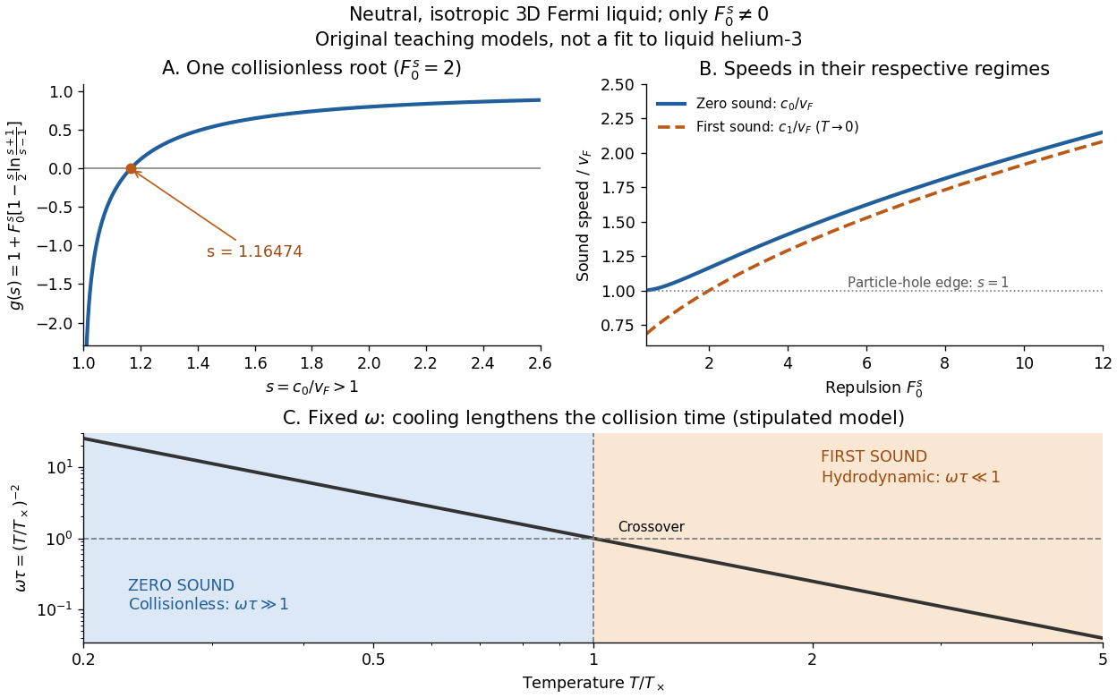
For the figure's stipulated law , cooling from to changes from to , without changing the driving angular frequency. The crossover temperature is defined by . Calling zero sound a high-frequency mode therefore means high relative to the collision rate , while its excitation energy must still remain within the low-energy domain of the Fermi liquid.
Isotropic zero-sound model Created 2026-10-18 Updated 2026-10-20
Consider a neutral, isotropic, unpolarized three-dimensional spin-one-half Fermi liquid, with only nonzero. A longitudinal density wave with angular frequency and wavevector magnitude has . The collisionless angular equation for the energy displacement of the Fermi surface isAveraging givesThe bracket decreases from infinity to zero on : each gives one undamped root above the small- particle-hole continuum.[ref]
For an original example, gives . Since here, the Principle of Galilean relativity gives and taking the hydrodynamic limit before gives . Stipulating gives and . These are model choices, not helium-3 measurements. At large , expanding the logarithm gives ; for small positive , the root approaches exponentially closely, so numerical resolution matters. A charged electron liquid needs its long-range interaction included; this neutral model is not its long-wavelength density mode.

Zero-point motion Created 2026-10-18 Updated 2026-11-05
Zero-point motion is the nonzero quantum fluctuation of position and momentum in a system's ground state. For a quantum harmonic oscillator, the ground state has energy and nonzero position and momentum variances even at zero temperature. It does not represent a thermal mixture and need not carry entropy. The large zero-point motion of light helium atoms helps explain why helium can remain a liquid at low pressure even as temperature approaches absolute zero.
Let be a bounded harmonic function in a bounded connected smooth planar region, with zero continuous boundary limits except at finitely many points. Then . This extends zero-boundary harmonic uniqueness to bounded solutions with isolated boundary exceptions, without assuming their initial Dirichlet energy is finite.
Choose within distance of each exceptional point, beyond distance , and interpolate linearly in the logarithm of distance. Each annular transition has . Apply the divergence theorem to the equation multiplied by . The ordinary boundary terms vanish, and the Cauchy-Schwarz inequality givesEvery fixed compact subset eventually has , so the gradient vanishes everywhere. The nonexceptional boundary data then fix the constant to zero. Differences of bounded harmonic extensions with identical piecewise continuous data satisfy this hypothesis. The individual extensions can have infinite Dirichlet energy at a jump; the cutoff argument avoids applying an unjustified finite-energy identity to them.
Zeeman slower resonance tracking 2026-10-18
A Zeeman slower prepares a slow beam for capture; a narrow longitudinal velocity group is not by itself a cold three-dimensional cloud. The historical apparatus measured slowed-beam velocities with a separate fluorescence probe scanned in frequency, just after switching off the slowing beam. This avoided simultaneous-beam complications.[ref]
For an original resonance-tracking calculation, let atoms travel along with and the slowing beam along , so its atom-frame angular frequency is . Approximate the selected cycling transition by on one field branch; is its signed angular frequency shift per unit magnetic field. A multilevel atom may require a nonlinear outside that branch. Maintaining a chosen effective laser detuning requiresFor chosen constant deceleration magnitude , gives and length . Substitution supplies a square-root magnetic field profile, plus a constant offset. The signs follow from the specified directions; reversing the selected transition's magnetic slope reverses the required field variation.
As a hypothetical design, take , and . The required length is and flight time . For chosen and , photon recoil velocity implies roughly directed absorption events. The mean required scattering rate is about . This budget must lie below the available scattering rate, with margin for capture and intensity variation. Optical pumping into unwanted hyperfine structure or magnetic sublevels can interrupt the cycle. Longitudinal slowing, transverse recoil heating and final cloud temperature are separate quantities.
There are unlisted articles, also show them or only show them.