
Proof stress 2026-10-18
An offset proof stress is defined by the intersection of a loading curve with a line parallel to its initial linear elasticity response but shifted by a specified engineering strain. A 0.2 percent convention uses the line , with Young's modulus .
Inelastic X-ray scattering Created 2026-10-18 Updated 2026-11-05
Inelastic X-ray scattering measures energy and momentum transferred from X-rays to matter. With sufficiently high energy resolution, it can map a phonon dispersion relation by measuring inelastic peaks at different momentum transfers. Crystal momentum is determined modulo a reciprocal lattice vector.
William Lawrence Bragg's 1913 structure paper connects a slit-selected beam, an oriented crystal and an ionization chamber to strength-versus-angle curves. Repeated sine ratios and matching absorption coefficients identify common radiation. Narrower slits resolve blended lines. Absolute wavelengths remain undetermined there; intercrystal comparisons first give relative scales. The Bragg crystal reflection experiment of 1913 covers the alignment controls.[ref]
The Structure of Some Crystals as Indicated by their Diffraction of X-rays by William Lawrence Bragg. pp. 268–272, especially Fig. 16: angular ionization scans, order/absorption comparison, slit resolution and wavelength-scale limitation
William Henry Bragg's 1915 Bakerian lecture, X-rays and Crystal Structure, separates the geometric and intensity arguments. Its Figure 9 compares reflection positions and strengths from three sodium chloride orientations; odd and even diffraction orders differ in strength along one orientation. The interpretation uses alternating scattering layers. Later, the calcite example identifies an internal oxygen coordinate that symmetry alone cannot fix. Improved wave intensity measurements revise a previously rough estimate. Thus a lattice assignment can precede determination of positions inside the unit cell; intensity interpretation also has experimental and theoretical limits. This is the father's 1915 lecture, distinct from the joint 1913 reflection paper.[ref]
Phase problem 2026-10-18
The phase problem is the loss of the wave phases of the crystal basis structure factors when an experiment records their squared magnitudes. Write . A Fourier series reconstruction of a periodic electron density uses both and , whereas an ordinary wave intensity measurement supplies only . Estimating the missing phases therefore needs additional constraints or measurements.[ref]
Phase problem. Online Dictionary of Crystallography by International Union of Crystallography; Definition: missing structure-factor phases prevent reconstruction of atomic positions; Methods of solution: estimates are tested against observations
There is also an unavoidable choice of origin. Translating all motif positions by the same fractional crystal coordinate vector multiplies by without changing . The physical arrangement is unchanged. A reconstructed coordinate list must therefore distinguish a coordinate convention from information actually recovered from the measurements.
Basis intensities and phase ambiguity 2026-10-18
Keep the cubic translations above, but attach an atomic basis with A at fractional crystal coordinates and B at . Stipulate real, angle-independent relative scattering amplitudes and . Neglect wave absorption, repeated crystal scattering and thermal motion. This is a point-scatterer model under the Born approximation, not a claim about the scattering strengths of named elements. Its crystal basis structure factor isHere is a dimensionless squared motif amplitude. Comparing it with measured integrated wave intensities requires the experimental geometry and detector response as well. The algebra follows directly by multiplying by its complex conjugate; the cross term records wave interference between the two sites.
With , reflections with even have , whereas odd gives , a ratio of . With , the first four values instead are . Their geometrically possible positions are unchanged, although their strengths change. For equal stipulated amplitudes and , the odd- amplitude vanishes exactly: an example of a systematic absence. Different motif weights can thus expose a repeat that equal weights conceal.
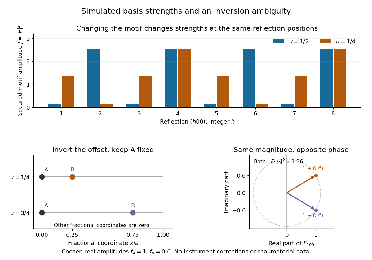
The motif changes intensities, while inversion can preserve them
. Original point-scatterer simulations with and . Top: the same reflection labels have different squared motif amplitudes for and . Bottom left: moving B from to inverts its offset modulo a translation. Bottom right: the two crystal basis structure factors are complex conjugates, , with the same squared modulus . No detector profiles or real-material measurements are plotted. Details.
The same formula also proves an ambiguity: and give identical for every integer , because . Yet changes from to , reversing its wave phase. This particular ambiguity is inversion of the motif; it does not prove that these two simple motifs are distinct chemical substances. The conclusion is conditional on the stipulated real scattering amplitudes.
Choose an original simulated model: a primitive cubic lattice with one identical point scatterer per primitive unit cell, edge , and incident X-ray wavelength . These are stipulated lengths, not measurements of sodium chloride. Suppose orientation information has already assigned the two observed reflections the Miller indices and . The detector deflection is , where is the Bragg angle.
Use the existing interplanar spacing formula and Bragg's law, with higher diffraction orders absorbed into the reflection indices:The simulated reflection has , hence . The reflection has , hence . Their squared sines are and , in ratio . Substituting the unrounded angles independently givesAgreement tests a proposed indexing and scale together; disagreement would prompt checks of the indexing, wavelength, angular zero, or the assumed unit cell geometry.
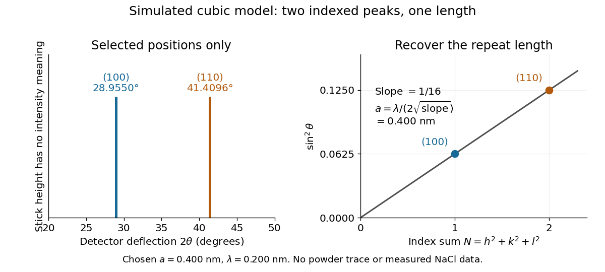
Two indexed reflections recover the same cubic repeat length
. Original simulation with and . Left: selected and positions on a detector-deflection axis; equal stick heights are only markers. Right: their squared sines lie on the line of slope . These are selected reflections, not a complete scan, a powder trace, or measured sodium chloride data. Details.
Two peak positions alone do not establish the indexing. Assigning the same two angles to and would give and instead. More reflections, orientation information and systematic absences help discriminate such assignments. An unobserved reflection can be inaccessible, weak or extinguished by the atomic basis; absence is not automatically evidence for a larger interplanar spacing.
Absolute scale also requires measurement calibration of the wavelength. To first order, differentiation of the inferred length giveswith angular changes in radians. A stipulated detector-zero error , with correct wavelength, biases the first inferred edge downward by approximately and the second by . A common angular offset therefore need not cancel when two inferred lengths are compared. These are model sensitivity estimates, not historical instrument uncertainties.
Grazing-incidence X-ray optics 2026-10-18
Grazing-incidence X-ray optics redirect X-rays by shallow specular reflections along mirror surfaces. Riccardo Giacconi's lecture describes coaxial paraboloidal and hyperboloidal mirrors using two reflections, and the later Einstein observatory's imaging capability. Focusing separates collecting area from detector area: the collected source signal can remain large while the detector background is drawn from a smaller region.[ref]
An ideal lossless geometrical optics calculation explains the shallow angle. Take vacuum refractive index one and a material with real refractive index , where . Let be the grazing angle measured from the surface. Snell's law written for angles from the normal requires . A propagating transmitted ray exists only if . Thus the ideal threshold isThe last step uses the Taylor series . For a chosen , radians, or . Absorption makes the refractive index complex and softens this ideal threshold; surface roughness and alignment errors also reduce throughput or worsen the point spread function. These are reasons to calibrate X-ray effective area and angular resolution, rather than assume that reflection is perfect.
The benefit can be quantified without specifying a historical telescope. Suppose a source retains fraction of its counts inside an extraction region, while a uniform detector background contributes counts over detector area . In the background-dominated limit of the same independent on-off model,Reducing by a factor of 100 at fixed and X-ray effective area improves this ideal ratio tenfold. A collimator restricts admitted directions; focusing optics bring selected rays together. An image also separates nearby sources and identifies clean background regions, connecting optical design directly to a better constrained inverse problem.
X-ray effective area 2026-10-18
X-ray effective area is the area that converts an incident photon arrival rate per unit area into an accepted count rate. For a fixed direction and a sufficiently narrow energy interval, writeHere is projected geometric area, is transmittance through windows or optics, is quantum efficiency, is the probability that a detected source event passes event selection, and is live observing time. is an expected value, not a guarantee of an integer count. Multiplication follows by counting incident photons over area and time, then applying the successive conditional acceptance probabilities. Live time already excludes intervals when the instrument cannot record events; multiplying by a live-time fraction again would count the same loss twice.
For an invented narrow-band example, choose , , , and . Then . A source with observed for gives . here counts photons; converting it into observed radiative flux requires their energies. If all have energy , the corresponding radiative flux is .
Diffuse X-ray background 2026-10-18
Diffuse X-ray background is X-ray emission spread over the instrument's observed sky rather than assigned to a single resolved source. Diffuse appearance at finite angular resolution does not prove emission by a continuous medium: many unresolved point-like astronomical sources can also give a smooth signal. Instrumental background is a separate contribution, even though both enter measured counts.
In 1962, Riccardo Giacconi and colleagues flew three Geiger counters to search for lunar X-ray fluorescence. Different mica thicknesses tested penetration; lampblack blocked ultraviolet. Each counter sat in an anticoincidence detector using a scintillation counter to reject cosmic rays. There was no mechanical collimator. Rotation scanned the sky; optical sensors supplied orientation.[ref]
Evidence for x Rays From Sources Outside the Solar System by Riccardo Giacconi and others. pp. 439–440, apparatus and readout
Counts were sorted by azimuth; a faulty counter and tumbling descent data were excluded. A directional peak lay above a diffuse component. Window, altitude and angular responses tested X-rays against charged particles; the Moon's nondetection checked optical leakage. The authors argued for an origin outside the Solar system, while residual cosmic ray background was not directly measured and source size, position and spectrum remained assumption-dependent.[ref]
Evidence for x Rays From Sources Outside the Solar System by Riccardo Giacconi and others. pp. 440–443, Figs. 1–4 and concluding limitations
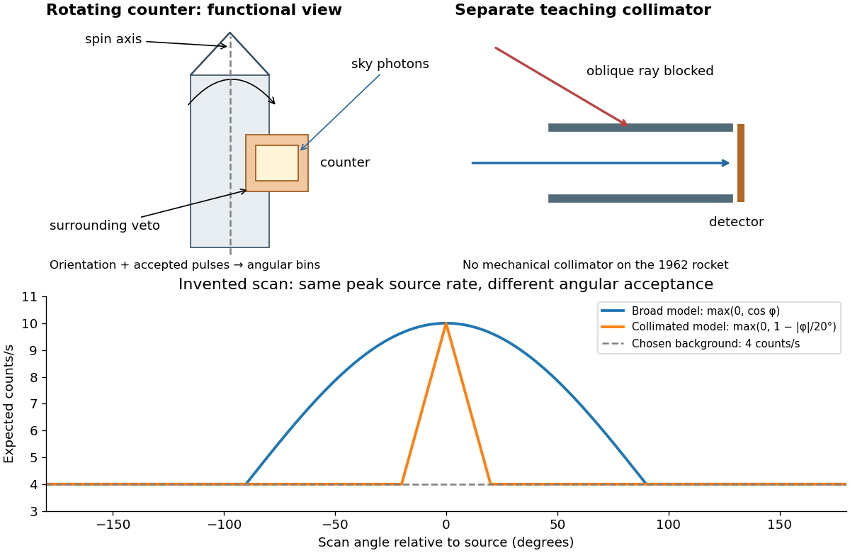

A simple original forward problem makes the distinction precise. Let be the scan azimuth, let be a dimensionless directional response with maximum one, let be a source's band-integrated photon arrival rate per unit area, let be its on-axis X-ray effective area, and let be a constant accepted background rate. The expected rate isFor a broad illustrative response , the full width at half maximum is : at . For a one-dimensional ideal collimator model , the full width at half maximum is . Choosing narrows the response sixfold without focusing any additional photons. These are teaching response functions, not reconstructions of the rocket's window transmission or geometry. A narrower scan peak can reflect the instrument response even when the source is unresolved.
Cosmic X-ray source Created 2026-10-18 Updated 2026-11-05
A cosmic X-ray source is an astronomical emitter detected through its X-rays. Hot plasma, energetic particles and matter falling into deep gravitational potentials can produce such radiation, so detection alone does not identify a black hole or one unique emission mechanism.
A useful observation proceeds from an excess of detector events to a sky location, spectrum and light curve. Background rejection and response calibration determine which incident photons could have produced those events. The 1962 rocket discovery of cosmic X-ray sources illustrates how a scanning detector and an independent orientation measurement can establish a celestial signal without forming an ordinary optical image.
Radiography Created 2026-10-18 Updated 2026-11-05
Radiography forms an image from spatially resolved transmission of X-rays or other penetrating radiation. A source illuminates the object, and a detector on the other side records how much radiation reaches each position. Variations in attenuation make internal differences observable without cutting the object.
A thicker region and a more strongly absorbing material can give similar transmission, so one projection does not uniquely determine composition or three-dimensional shape. Unwanted scattering reduces image contrast by adding radiation that did not follow the intended straight path. A reference exposure measures source and detector nonuniformity; multiple viewing directions provide additional geometric information.
X-ray attenuation 2026-10-18
For a narrow beam of monoenergetic photons crossing homogeneous material of thickness , the uncollided wave intensity obeys . Here is the linear attenuation coefficient, counting removal from the incident beam by photon absorption and scattering of light. It depends on photon energy and material; it is not universally independent of energy.[ref]
2. The Mass Attenuation Coefficient. Tables of X-Ray Mass Attenuation Coefficients and Mass Energy-Absorption Coefficients by John H. Hubbell and Stephen M. Seltzer; NIST, X-Ray Mass Attenuation Coefficients, §2, Eq. (1), narrow monoenergetic beam and interaction contributions
An original derivation makes the model explicit. If each thin layer removes fraction of the surviving beam, with the same throughout, thenThus equal added thicknesses multiply transmission by the same factor. The ordinary differential equation describes uncollided beam survival. To test it with a detector, keep source output, distance, selected photon energy band and detector response fixed. Use a collimator and suitable detector acceptance to exclude scattering of light into the detector. Subtract background, measure an empty-path reference, and keep the detector in its linear operating range. A changing source distance adds geometric dilution and is not an attenuation measurement at fixed geometry.
For a stipulated example, take and . Transmission is . If the empty-path detector rate is , including background , the model predicts sample rate . Recover transmission as ; the raw ratio is biased. These chosen values are a calculation, not measurements of a particular material or a historical apparatus.
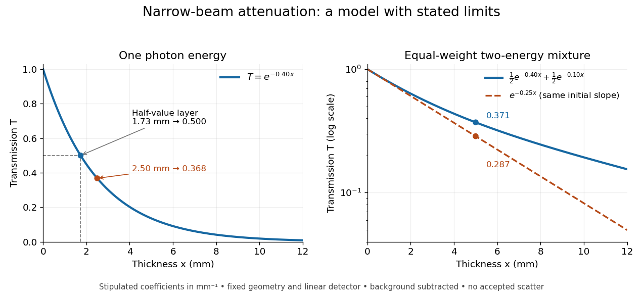
When X-ray transmission is exponential, and when spectral mixing bends it
. Original calculated examples, with stipulated linear attenuation coefficients in inverse millimetres. The left panel uses one photon energy and marks and the half-value layer. The right panel compares an equal-weight mixture of two photon energies with the exponential having the same initial slope. A logarithmic vertical axis turns a single exponential into a straight line. Neither curve is fitted to measured material data. Details.
X-ray tube Created 2026-10-18 Updated 2026-10-20
An X-ray tube accelerates electrons from a negative cathode to a positive target anode. A heated cathode supplies electrons by thermionic emission; the evacuated envelope limits collisions before the target. This differs from the gas-discharge tube in the Röntgen X-ray discovery experiment.[ref]
Chapter 5: X-Ray Production (teaching slides) by K. P. Maher. Diagnostic Radiology Physics: A Handbook for Teachers and Students; IAEA, Chapter 5: X-Ray Production, §§5.2–5.3.2; authored teaching slides, inspected transcription
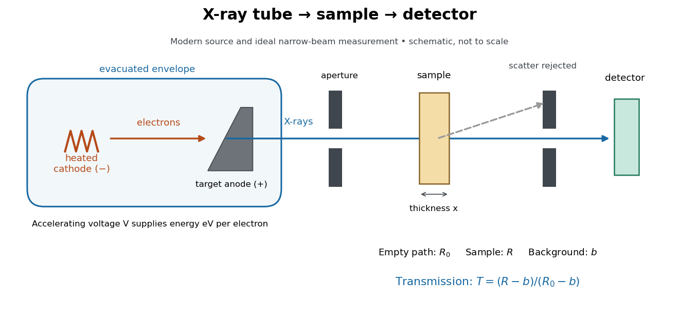

In bremsstrahlung, an electron changes velocity in the target's electric fields, emitting a photon while losing kinetic energy. Different encounters allow a continuous range of transferred energies. This is distinct from the discrete electronic transitions producing Characteristic X-rays.
Changing the accelerating voltage changes the available kinetic energy per electron and the X-ray tube cutoff. Changing the number of arriving electrons changes the number of opportunities for photon emission. These are distinct controls: a larger electric current does not by itself give each electron more energy. For an original idealized budget, and tube electric current give electrical power and arrival rate , where is the elementary charge. This is input power, not emitted X-ray power; obtaining the latter requires a conversion efficiency.
Bothe-Geiger coincidence experiment Created 2026-10-18 Updated 2026-10-20
In 1924–1925, Walther Bothe and Hans Geiger tested event-level Compton scattering correlations against the statistical conservation proposed by BKS theory.[ref]
The Coincidence Method by Walther Bothe. The coincidence method, pp. 271–273
Needle Geiger counters shared a wall. X-rays passed beside it through hydrogen; recoil electrons registered in one counter and scattered photons triggered electron release in the other. Photographic records resolved approximately .[ref]
The Coincidence Method by Walther Bothe. p. 272: apparatus and timing
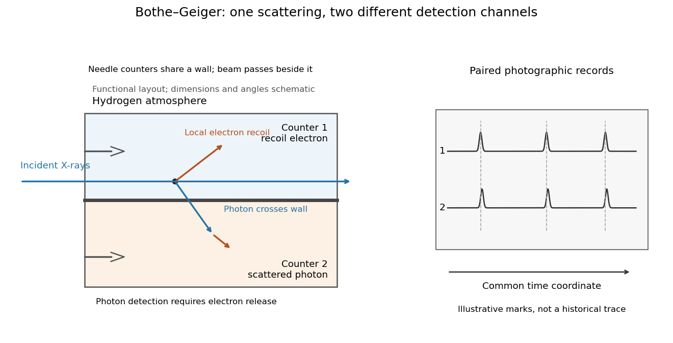
Two detection channels in the Bothe-Geiger coincidence experiment
. Original functional schematic based on Bothe's account; dimensions, angles and trace marks are illustrative. The common wall separates the counter regions; the direct beam avoids it. The drawing specifies neither wall material nor chamber shape. Photon detection requires electron release. Both records share a time coordinate. Details.
The coincidence excess matched paired-emission expectations. Bothe distinguishes a later directional test from this timing experiment.[ref]
The two channels have different physical roles. The first responds to the local recoil electron's ionization. The second converts a scattered photon into an electron response, as in the photoelectric effect. A large counter signal is an amplified indication of an interaction, not a direct measurement of the incoming photon's energy. The detection efficiency and accepted directions determine how many genuine partners can be seen. Consequently, failure to record every partner is compatible with paired production.
The relevant distinction is between an average balance and a balance in each event. For an initially stationary free electron, Compton recoil kinematics givesHere are incident and scattered photon energies, is recoil kinetic energy, and is electron momentum. These are paired constraints, not just equations between averages over unrelated detections. Summing correctly paired events preserves the equations; throwing away the pair identities loses information. Two samples can have identical separate energy distributions while differing in their joint probability distribution.
The experiment therefore supplied evidence for the event association required by photon recoil, rather than weighing both outgoing energies in every event. A statistically established excess above accidental coincidences matters; one near-simultaneous pair cannot establish the association. It also cannot by itself settle every question about wave-particle duality.
Preparation, readout and background checks address different failure modes. The direct beam must avoid the second counter, and the counter boundary must prevent a recoil electron from masquerading as its own photon partner. Separate-channel rates constrain accidental coincidences; common disturbances or electrical coupling could instead create a correlated instrumental background. A useful diagnostic is to displace one record in time: under a stationary process assumption, unrelated-pair expectations persist while prompt partners separate. This is the explanatory control modeled below, not an assertion that Bothe performed that particular record-shifting procedure. A background estimate and a statistical comparison are essential to the inference.
The existing coincidence circuit article explains electronic selection, and accidental coincidence derives the accepted-window background. Here pairing can be understood directly from the two recorded time sequences, without imposing a modern detector trigger on the historical readout.
Röntgen X-ray discovery experiment 2026-10-18
Wilhelm Conrad Röntgen's 1895 first communication describes an induction coil driving an evacuated gas-discharge tube, enclosed in black cardboard in darkness. A paper screen coated with barium platinocyanide showed fluorescence even with its uncoated side facing the tube, visible two metres away. The covering excluded ordinary illumination.[ref]
On a New Kind of Rays by Wilhelm Conrad Röntgen. Röntgen, On a New Kind of Rays, §§1–2; inspected reprint p. 153
He interposed materials: a thousand-page book transmitted; lead was practically opaque. A stepped stack of foil produced a photographic plate record. Different materials were not equivalent at equal density and thickness. Photographic plates checked visual observations while remaining covered against ordinary illumination.[ref]
On a New Kind of Rays by Wilhelm Conrad Röntgen. First communication, §§2–6; reprint pp. 153–154: absorption tests and photographic controls
Section 14 lists photographs of hand bones, wire on a bobbin, boxed weights, an enclosed compass, and a lead-painted door. It does not identify the hand's owner. Magnetic deflection moved the cathode ray impact point and thus the source, without bending the emerging X-rays. Their nature remained unsettled.[ref]
On a New Kind of Rays by Wilhelm Conrad Röntgen. First communication, §§11–14 and 17; reprint pp. 156–157
The observations belong to 1895; the contemporary English translation appeared in Nature on 23 January 1896.[ref]
On a New Kind of Rays by Wilhelm Conrad Röntgen. Catalogue, On a new kind of rays: notes identify the Nature translation and its publication date
The experimental logic separates production, transmission and detection. A visibly opaque covering can transmit X-rays; fluorescence then converts deposited energy into visible light. A shadow measures a difference between paths through an object, rather than a direct view of its surface. Neither a screen's brightness nor photographic darkness alone measures an absolute X-ray energy or establishes the X-ray attenuation law below. There are unlisted articles, also show them or only show them.