
For a weakly damped well, quantizing the conservative part of current-biased Josephson phase dynamics gives the local Hamiltonian operatorThe tilted potential energy is unbounded downhill. Its trapped energy levels are therefore long-lived resonances with escape lifetimes, rather than globally bound stationary states. Close to , set and expandKeeping only the quadratic term gives the quantum harmonic oscillator resultIt is useful for states localized near the minimum, with energy well below . It does not count all the resonances accurately near escape. The omitted terms make successive spacings unequal. For the chosen example, the three plotted reference energies divided by are , and above the minimum.
A small microwave bias contributes . A one-photon transition between energy levels is resonant when . Exciting a higher energy level can strongly increase its escape probability. Measuring microwave absorption indirectly through escape therefore connects an invisible quantum phase state to a visible electric potential difference. A classical oscillation can also show resonance, so the mere existence of one peak is insufficient: the bias dependence and resolved unequal spacings are the discriminating predictions.
Tilted Josephson washboard potential 2026-10-18
At fixed positive bias ratio with , the Josephson coupling energy and work of the ideal bias source combine intoThis is the effective potential energy for an unwrapped Gauge-invariant Josephson phase; it includes the bias source and decreases by on advancing one period. A local minimum and the adjacent downhill barrier areTo verify the barrier, solve , select and , and subtract their potential energies. The small-oscillation angular frequency is fixed by the curvature:Thus the barrier and oscillation frequency both vanish as , but with different powers. For , expanding and givesThe first approximation is for a nearly critical bias. At the exact downhill barrier is ; at there is no confining local minimum in this model.
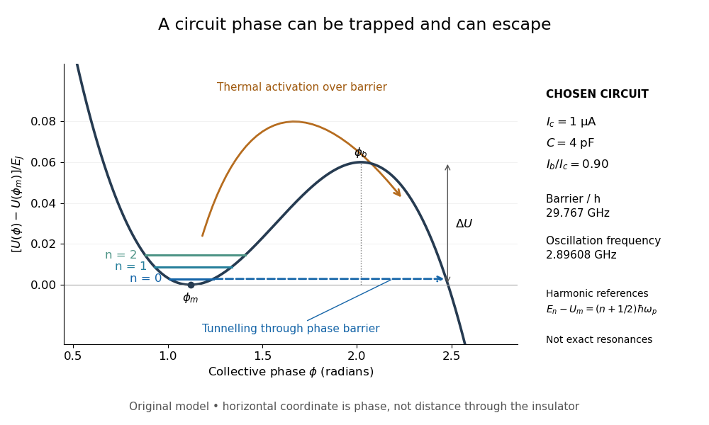
A tilted phase potential confines low energy levels and permits escape
. Original chosen model with , and . Three horizontal lines are quantum harmonic oscillator approximations , for ; they are not exact energy levels or measured data. The horizontal axis is a quantum phase, not distance through an insulator. Arrows distinguish over-barrier thermal activation and below-barrier quantum tunnelling. Details.For those stipulated parameters, direct evaluation gives , , and . Hence . The nearly critical barrier approximation gives , about below the exact result. These are original circuit calculations, not parameters assigned to the historical samples.
Formal hole count in a cuprate Created 2026-10-18 Updated 2026-10-20
For a chosen homogeneous composition , assign formal oxidation states to lanthanum, to barium and to oxygen. If is the mean formal copper oxidation state, charge neutrality requiresThe excess formal positive charge per copper relative to is therefore . For stipulated and , it is ; at , it is zero. These are bookkeeping examples, not measurements of mobile carriers. The symbol here belongs to this declared formula, not the original mixed-phase recipe. A whole-pellet elemental ratio cannot simply be assigned to each constituent phase.
Charge neutrality alone does not locate holes. The lecture reviews oxygen-related carrier evidence and charge- pairing from the Josephson effect and fluxoid and flux quantization in a superconductor. Pair charge does not establish phonon-mediated BCS theory for cuprate superconductors.[ref]
Perovskite-type oxides: The new approach to high-Tc superconductivity by Johannes Georg Bednorz and Karl Alexander Müller. Part 2, pp.444–446, 450; pairing, carriers and mechanism
Integrated cumulative distribution function on a bounded interval Created 2026-10-18 Updated 2026-11-05
If a random variable takes values in , its cumulative distribution function satisfiesIndeed for every outcome. Taking expected values and using Tonelli's theorem proves the formula, including when the probability distribution has atoms. For a probability density function , the same proof reverses the order in . Thus , restricted to , is a probability density function whenever . The reflected construction using has normalising constant and is closely related to an integrated tail distribution.
X-ray diffraction 2026-10-18
X-ray diffraction is the angular redistribution of X-ray wave intensity through wave interference between scattered waves. In a crystal structure, repeated lattice translations select discrete outgoing directions by the Laue equations. A photographic plate can therefore turn invisible atomic periodicity into a visible constellation of spots. Their geometry constrains the Bravais lattice and its orientation; their wave intensities also depend on the crystal basis structure factor. Determining atomic positions belongs to X-ray crystallography and requires more information than recognizing a spot pattern.
The Laue X-ray diffraction experiment of 1912 established this phenomenon experimentally. The Laue method uses a fixed crystal structure with a range of incident wavelengths; the Bragg crystal reflection experiment of 1913 instead measured angularly resolved signals with a moving detector. These are different ways of finding the same coherent elastic scattering directions.
Systematic absence Created 2026-10-18 Updated 2026-11-05
A systematic absence is a class of diffraction reflections forced to vanish by symmetry or a repeated structural motif, rather than merely being weak by accident. It follows from exact cancellation in a crystal lattice structure factor or crystal basis structure factor within the stated scattering model.
For identical body-centering-related scatterers, vanishes whenever is odd. Changing the motif can lift the cancellation, as in chemical ordering and body-centering extinction. Additional effects such as unequal species amplitudes, disorder or multiple scattering can also produce intensity where a simplified model predicts zero. Reflection conditions therefore help infer structure, but an observed weak or missing spot needs a measurement and model qualification before it is treated as an exact symmetry statement.
Thermal boundary resistance 2026-10-18
Thermal boundary resistance describes a temperature drop between the two sides of a material interface carrying heat flux. Efficient thermal conduction within each material does not guarantee efficient heat transfer between them. The solid–helium case is Kapitza resistance; the broader concept also includes solid–solid interfaces. [ref]
Let and be the temperatures extrapolated to the interface from its solid and liquid sides, each treated as internally in thermal equilibrium. For uniform normal heat flux through area , define the finite-drop, area-specific thermal resistance and the resistance of the whole interface byThe macroscopic jump represents an unresolved interfacial region; it is not a claim that one point has two equilibrium temperatures. At nonzero heat flux, the two sides are outside mutual thermal equilibrium. A measured difference between distant thermometers also contains bulk temperature gradients, which must be measured or bounded before assigning all of it to the interface.
An energy balance explains why a temperature jump can coexist with continuous heat flux. For a stationary interfacial region with no local work or heat source,The first law of thermodynamics therefore requires in a steady state. It does not require . For a heated sample with electrical power , an independently determined outward parasitic loss and no other inputs,Here is the heater's electric potential difference and its electric current. Subtracting a lead loss means subtracting power before dividing by area; is not the total heating power. Unknown losses and stored internal energy prevent that simple steady inference.
For a one-dimensional comparison, put an interface between two slabs with the same area , positive constant thermal conductivities and lengths . Neglect side losses. Integrating Fourier's law across each slab givesThus, for a linear interface with constant , the series result isThese slab formulas are a chosen thermal conduction model, not a bulk transport law for moving liquid helium. If the interface law is nonlinear, substitute its own relation between and into the preceding balance; a single constant resistance cannot describe every load. Increasing bulk thermal conductivity has diminishing benefit when the interfacial drop dominates. Increasing usable contact area reduces the whole-interface thermal resistance if the local interface law and the other conditions remain fixed.
Helium liquefaction 2026-10-18
Helium liquefaction converts helium gas into a collectable liquid. It creates a bath for investigating material properties at very low temperatures, including superconductivity. The central question is how the incoming specific enthalpy compares with the specific enthalpies of the outgoing liquid and vapor. The liquefaction enthalpy budget makes that comparison explicit; a temperature decrease by itself does not specify a liquid yield.
In a Joule-Thomson effect cooling stage, a throttling pressure drop approximately preserves enthalpy under the assumptions of the steady-flow energy balance. For an ideal gas, specific enthalpy depends only on temperature: with positive specific heat capacity at constant pressure, equal specific enthalpy means equal temperature. Thus its Joule-Thomson coefficient is zero. An ideal gas also supplies no liquid branch. Cooling by throttling depends on real gas properties; expansion is not an automatic source of refrigeration.
For a local drop , cools only where the Joule-Thomson coefficient is positive. Precooling must bring the real gas into a useful cooling region, with enough cooling to overcome unwanted heat transfer. A finite expansion can cross a Joule-Thomson inversion curve; its final state requires the full enthalpy balance, including phase coexistence if liquid forms. Kamerlingh Onnes's 1908 helium liquefaction experiment combined external precooling with regeneration to reach that regime. The Joule-Thomson effect article develops the throttling identities and their assumptions.
Cryostat Created 2026-10-18 Updated 2026-10-20
Delayed neutron-capture coincidence window 2026-10-18
Why not accept every delayed pulse? A longer window captures more genuine neutron capture signals, but also admits more accidental coincidences. Consider an original model with a capture waiting time following an exponential distribution of mean . Assume detection after a prompt signal accepts , with perfect time measurement and no lower cut. Integrating the normalized density givesThis assumes that moderation, competing capture channels, boundaries and electronic recovery can be represented or neglected in a single effective waiting-time model. It is not a fitted historical capture law.
Let independent prompt-like and delayed-like background streams have Poisson process rates and . The accidental coincidence pair rate in a directed window of full width is . Electronics producing at most one accepted delayed match per prompt instead give . These definitions coincide to first order when . Correlated backgrounds, such as one external neutron producing both a prompt recoil and a later capture, require separate controls; an independent-stream estimate cannot remove them.
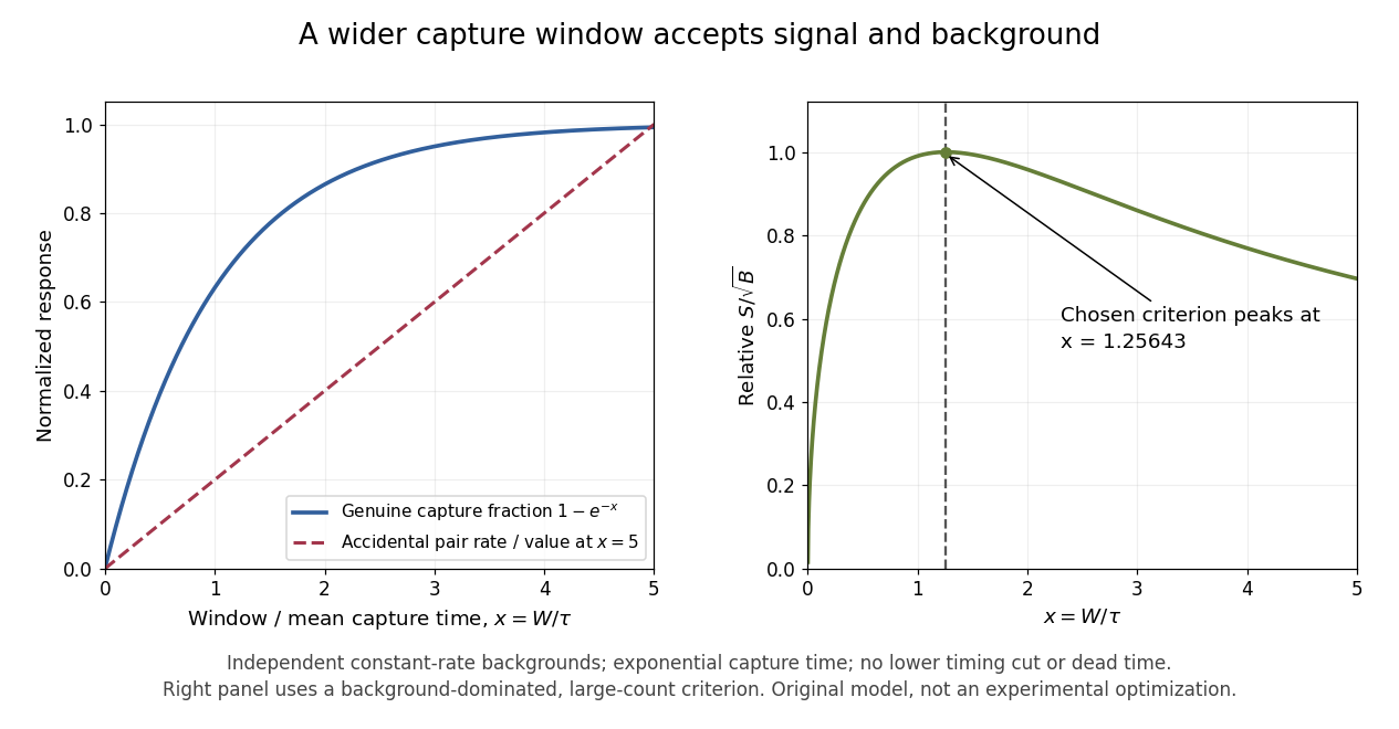
For chosen and , the accepted fraction is . With chosen and , the pair rate is , while the at-most-one rate is approximately . These are teaching parameters, not reported Savannah River rates. A measured uncorrelated background can be tested using displaced time windows; a reactor-off measurement addresses a different question and cannot by itself characterize every reactor-correlated background.
Inductance matrix 2026-10-18
An inductance matrix relates magnetic flux linkages to electric currents in a linear model of coupled inductors. For reciprocal two-coil coupling, . Its stored magnetic energy is . With , it is a positive-definite matrix exactly when . Equality is a singular limiting model requiring separate treatment.
Take the symmetric group and the subgroup of group order two. With the rightmost permutation applied first, its three left cosets areThe subscripts record the image of : every member of sends to . Because is the stabilizer subgroup of in the usual group action, is a bijection onto . It is an equivariant map, since . The coset action therefore becomes the familiar group action on three letters. In particular,
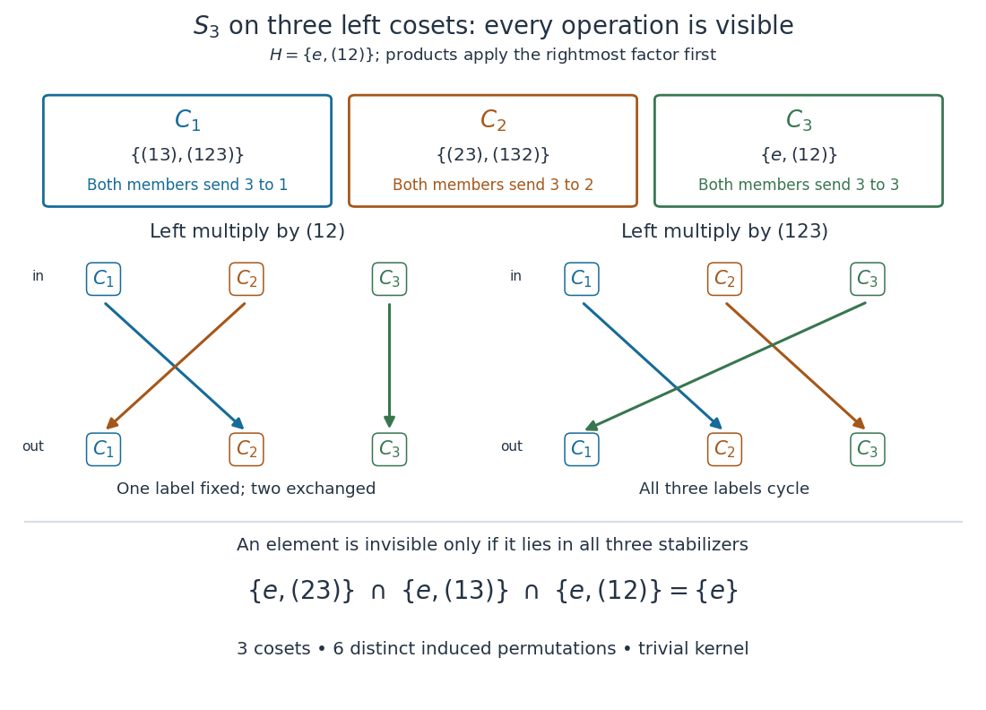
The three stabilizer subgroups areTheir intersection is , so the subgroup core and the group kernel are trivial. This proves that the coset action is a faithful group action even though every point has a nontrivial stabilizer subgroup. The orbit-stabilizer theorem reads , while the induced group homomorphism gives six distinct permutations of the three cosets. For example, and agree at , but disagree at ; inspecting one label would miss their difference.
The subgroup need not be a normal subgroup for the coset action to exist: . Here the group action is informative because the three conjugate stabilizer subgroups have no common nonidentity element. For the normal subgroup instead, nonfaithful coset action of the symmetric group on three letters shows that only the sign of a permutation survives.
Use local east, north, and up unit vectors , with . In a spherical-Earth approximation at geographical latitude , the angular velocity has components . Expanding the cross product for relative velocity givesThese are Coriolis acceleration components, not the total acceleration. For horizontal motion, the horizontal part is , where the Coriolis parameter is . Thus northward motion in the northern hemisphere has an eastward Coriolis acceleration, to the right of its velocity; in the southern hemisphere the horizontal turning is to the left. At the equator , but the full Coriolis acceleration need not vanish: vertical or eastward motion still couples through .
For a numerical example, take the Earth rotation rate , geographical latitude , and an initially northward relative velocity . Then
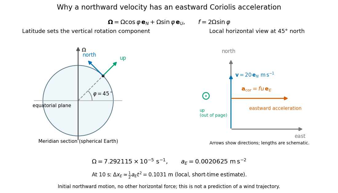
Latitude, local rotation geometry, and the scale of eastward Coriolis acceleration for northward motion
. Details. For a local, short-time estimate with no other horizontal force and zero initial eastward velocity, hold the initial northward velocity in the leading term: . At this gives about eastward. It assumes nearly fixed local axes and geographical latitude, negligible changes of height, and . It is not a complete wind trajectory: pressure gradients, friction, and evolving velocity must enter an atmospheric equation of motion. The effective gravity in a rotating frame already combines ordinary gravity with the steady terrestrial centrifugal acceleration.
Free particle in rotating coordinates 2026-10-18
Consider a ball moving horizontally with no net horizontal force in the laboratory. Treat its horizontal motion as that of a free particle: with constant . Axes rotating counterclockwise at constant angular velocity about the launch point assign it the positionThis is an exact rotation matrix transformation, with the axes coinciding at . Taking , , and gives the two views below. At , the laboratory position is , but the rotating position is approximately . Both assign the same distance from the origin.
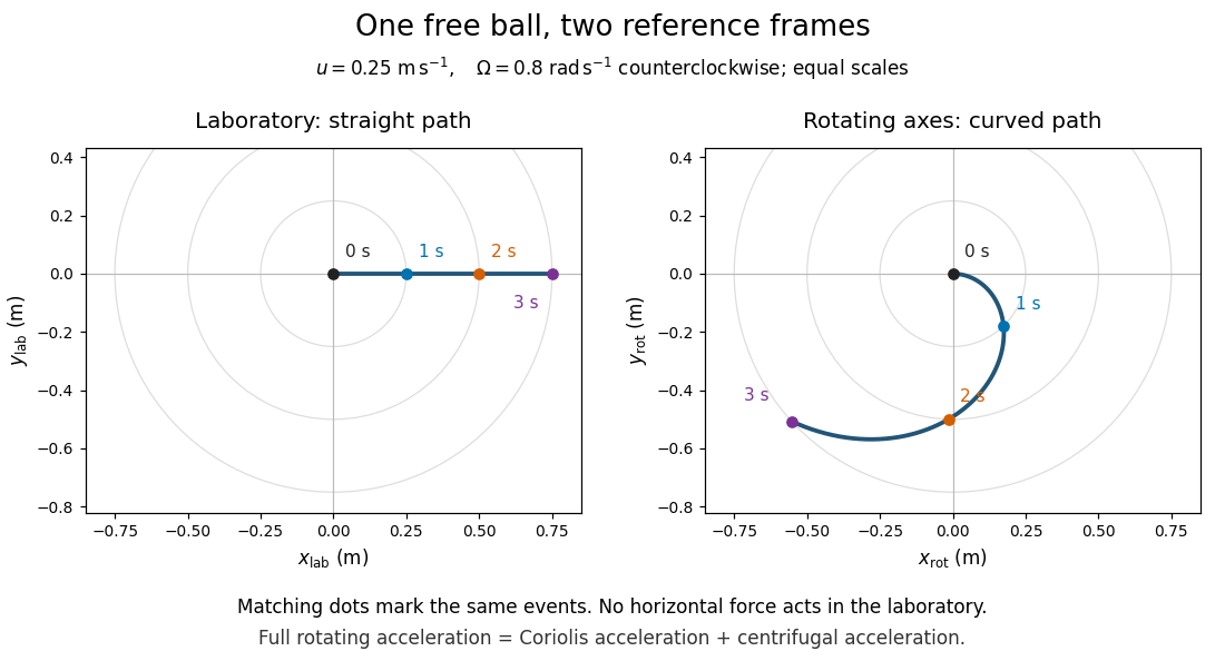


The entire rotating acceleration must include the centrifugal acceleration as well as the Coriolis acceleration. To see the balance explicitly, write and . Direct differentiation givesThe two apparent contributions areAt launch , so only the Coriolis acceleration contributes to the initial bending. Later the centrifugal acceleration also contributes; the full curved trajectory cannot be explained by keeping only the Coriolis force. In particular, grows even though the Coriolis force does no work: the rotating-frame kinetic energy increase is supplied by work from the centrifugal force. The laboratory kinetic energy remains .
SN 1987A Created 2026-10-18 Updated 2026-10-20
SN 1987A supplied a prompt terrestrial record of neutrino emission from a core-collapse supernova through its SN 1987A neutrino burst.[ref]
Nobel Lecture: Birth of neutrino astrophysics by Masatoshi Koshiba. p. 1015: supernova signal and collapse interpretation
Pairing gap Created 2026-10-18 Updated 2026-11-05
A pairing gap is an energy scale for fermionic excitations above a paired superfluid or superconductor ground state. In a simple isotropic paired system the quasiparticle dispersion has the form , where measures the unpaired single-particle energy relative to the chemical potential. A nonzero minimum gap gives exponentially small fermionic thermal occupations when . If the gap varies with direction and has nodes, gapless directions can instead produce power-law thermodynamics. Collective excitations must be counted separately from the gapped fermionic quasiparticles.
Self-convolution of a bilateral exponential Created 2026-10-18 Updated 2026-10-25
For and , split the convolution integral at and . The three contributions are , and . Evenness gives the displayed answer for all real .
With Fourier transform convention , one has . The convolution theorem and Fourier inversion theorem therefore yieldThe value at is . Multiplying by instead gives a normalized Laplace distribution; its self-convolution is the density .
Terms of a convergent series tend to zero Created 2026-10-18 Updated 2026-10-25
If the partial sums tend to a finite limit , then . Thus failure of the terms to tend to zero proves divergence. The converse is false: the harmonic series has terms tending to zero but diverges.
Quasi-static tether contraction 2026-10-18
For two equal point masses joined by a light tether of length , the central moment of inertia is . With conserved angular momentum , the rotational kinetic energy is . Slow, smooth contraction gives with the displayed leading tension. The exact radial correction is and , so the total work-energy theorem remains exact for non-quasi-static schedules too.
Conditional expectations algorithm cost 2026-10-18
Directly scanning all edges to evaluate each child of each of choices takes elementary operations, in Big O notation. There is a faster implementation. When assigning vertex , let and count its already assigned graph neighbours labelled zero and one. Contributions from edges not incident to are unchanged, and contributions from edges to unassigned graph neighbours stay for either choice. ThereforeChoose zero if , otherwise one: put on the side with fewer already assigned graph neighbours. With adjacency lists, scanning each vertex's list once costs operations overall and uses storage including the graph. These bounds count operations on labels and counters that fit in machine words of bits. Multiplying the conditional expectation cut formula by two also permits exact integer comparisons without rounding.
If is the size of a maximum cut, then . The constructed cut of a graph thus has size at least , an approximation ratio of in the maximization convention. The five-versus-six example illustrates the gap between this guarantee and exact optimization.
For a general randomized algorithm, the averaging proof alone does not establish efficient derandomization. One needs a polynomial number of commitments, an efficient way to find a suitable child at each step, and manageable representations and evaluation costs for the relevant conditional expectations. Those evaluations can themselves be hard. Enumerating all completions verifies this small example, but would take exponentially many assignments as grows. The polynomial-time algorithm here comes from the local conditional expectation cut formula, not from that enumeration.
There are unlisted articles, also show them or only show them.