
Conditional expectations cut example 2026-10-18
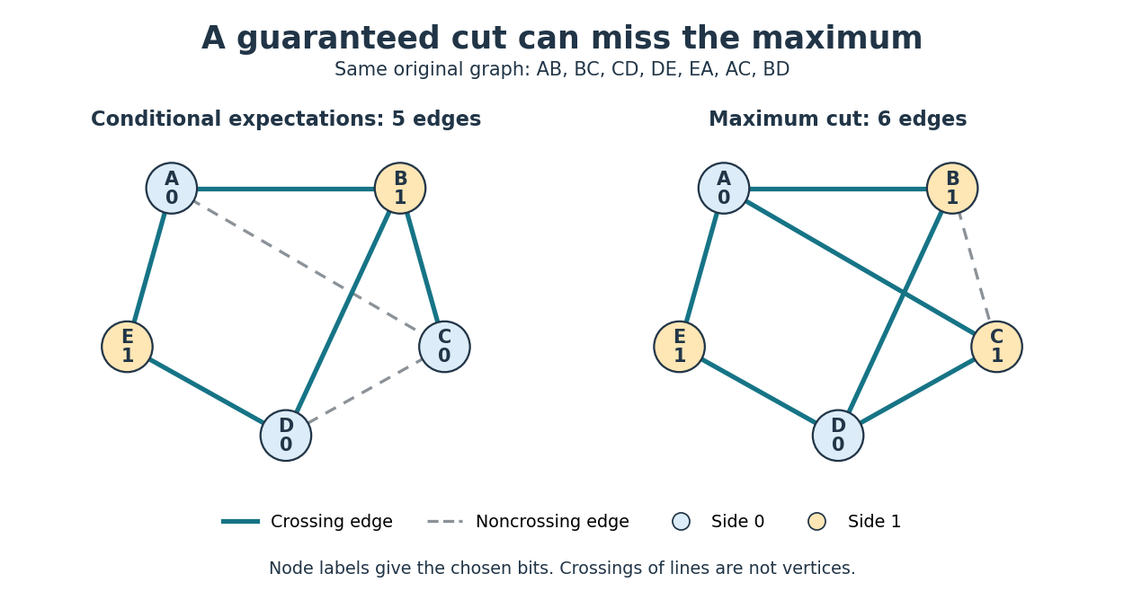
Consider the following original five-vertex simple graph, where denotes the undirected edge :Its seven edges give initial expected value . Use vertex order and choose zero whenever the two child conditional expectations tie.

The complete decision ledger is below. A prefix lists fixed labels in vertex order; all later labels remain hypothetically independent fair bits. Each candidate entry is the conditional expectation of the final cut of a graph, including the contribution of unresolved edges.
| Prefix before choice | Next vertex | Set to 0 | Set to 1 | Chosen label | Retained conditional expectation |
|---|---|---|---|---|---|
| Empty | |||||
For example, after , edge is fixed crossing and the other six edges are unresolved, giving . Setting fixes crossing and noncrossing, leaving four unresolved edges: . Setting instead fixes crossing and noncrossing, giving the same conditional expectation.
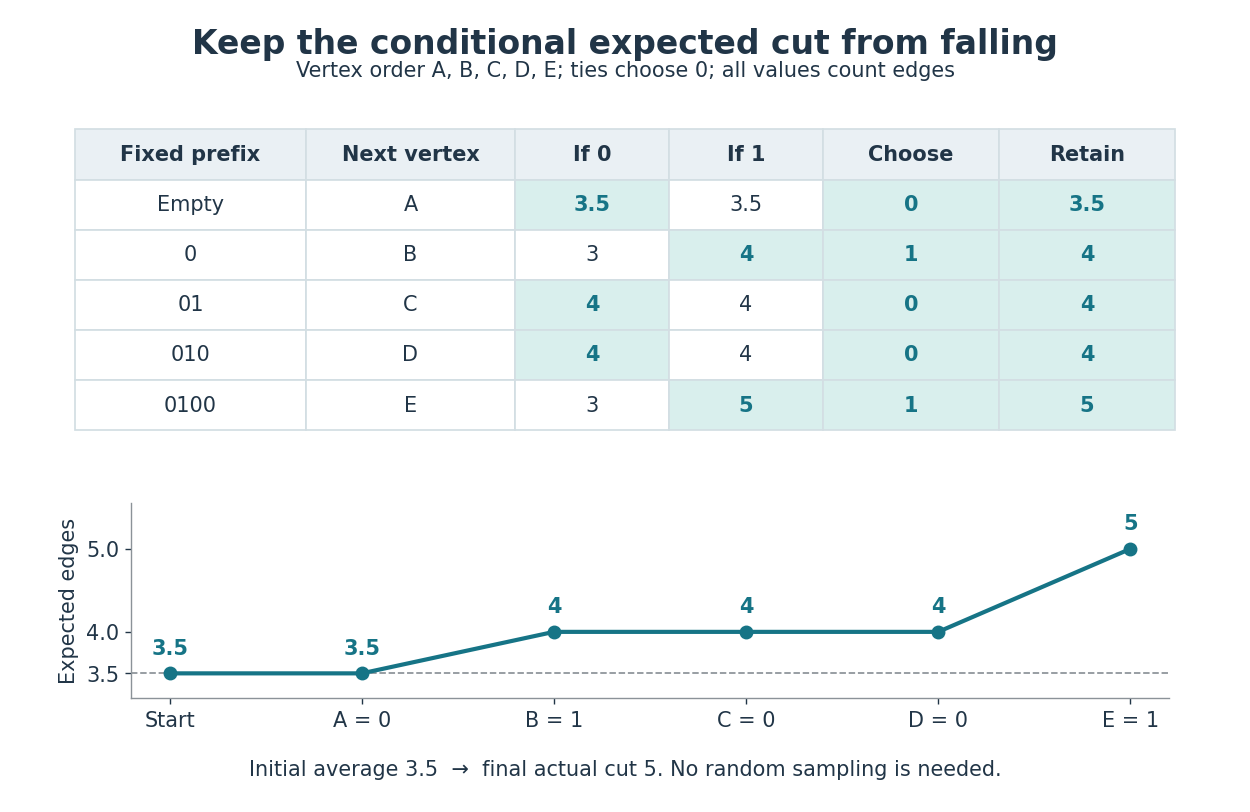
Conditional expected cut values along every chosen branch
. At each step, both candidate values are computed by the conditional expectation cut formula. The highlighted cell is chosen; ties choose zero. Below, the retained conditional expectation follows , starting before any label is fixed. The last value is the actual size of the resulting cut of a graph, rather than an average over remaining choices. Details.
The final labels are , so the two sides are and . The five crossing edges are ; do not cross. This exceeds , and hence also the rounded-up guarantee of four edges.
It is not a maximum cut. Labels cross all edges except , giving six. Seven are impossible because the triangle in a graph cannot have all three edges crossing a two-sided cut of a graph. An independent enumeration of all complete label assignments gives the following distribution, counting an assignment and its label-swapped counterpart separately:
| Size of cut of a graph | Number of label assignments |
|---|---|
The weighted sum is , so the average is , agreeing with linearity of expectation. Choosing in the earlier tie discards the remaining size-six completion while preserving the average of four. The method protects an expected value guarantee; it need not preserve the best possible completion.
Conditional expectation cut formula 2026-10-18
For any partial assignment , let count edges whose two endpoints are already fixed on opposite sides, and let count edges with at least one unassigned endpoint. Under the remaining independent fair bits,An edge with fixed equal labels contributes zero; fixed unequal labels contribute one. If one endpoint is unassigned, its fair bit disagrees with the fixed label with probability . If both endpoints are unassigned, their independent fair bits disagree with probability as well. Count each unresolved edge once, even when both endpoints are unassigned.
Process vertices in a fixed order. Evaluate the conditional expectation cut formula after setting the next label to zero and after setting it to one; retain the larger value, choosing zero on ties. The conditional expectation choice invariant ensures the final cut of a graph has size at least . This is a deterministic approximation algorithm for maximum cut.[ref]
Lecture notes on randomized approximation algorithms. CS 4820: Algorithms, Spring 2011; Cornell CS 4820, Lecture notes on randomized approximation algorithms, 2 May 2011, §1.1.2, printed pp. 2–3: conditional expectations, Algorithms 1–2 and the half-total-edge-weight guarantee; no individual byline stated
Paired logarithmic series with zero sum 2026-10-18
The terms at and are and its negative. Thus the partial sums ending at an odd index are zero, while those ending at equal . Considering both subsequences proves convergence of the full sequence of partial sums, not merely of grouped terms.
The paired sum of absolute values is . Since for , these pairs dominate , whose series diverges by comparison with the harmonic series. The original series therefore has conditional convergence with the displayed sum.
Concentration-blob size in a theta solvent Created 2026-10-18 Updated 2026-10-20
For an ideal chain inside a blob, and . Together with , this gives the displayed concentration-blob size. Under the site-volume approximation , and . The estimate describes local overlap rather than the full chain size and requires for a well-developed semidilute regime.
Optical extinction coefficient 2026-10-18
The imaginary part of the complex refractive index makes wave amplitude decay as . Since intensity is proportional to amplitude squared, its absorption coefficient is .
Real axis 2026-10-18
The real axis consists of the points of the complex plane whose imaginary part is zero. These points represent the real numbers.
Noncommutativity 2026-10-18
A binary operation is noncommutative if some pair of elements fails to commute. Thus reversing their order can change the result. The same operation may still have many commuting elements.
The 2000 experiment prepared optical pulses with a mode-locked laser and broadened them in an air-silica microstructure optical fiber. A wavelength-selective beam splitter separated red and blue light. A nonlinear crystal doubled the red branch; the blue branch received a known acousto-optic shift. A filter selected recombined light for an avalanche photodiode, supplying an electronic beat. Mirror translation controlled repetition frequency; mirror tilt controlled offset with coupled effects. Separate delayed-pulse interference tested programmed phase changes. Alternative envelope fits and unmatched optical reflections were examined as checks and limitations.[ref]
These readouts answer different questions. The electronic beat closes a feedback loop; changing its setpoint and checking the delayed-pulse phase tests whether that control reaches the optical waveform. Neither readout alone establishes the accuracy of an unknown optical frequency. That additionally requires a calibrated time reference, the correct tooth number and beat sign, and checks for missed cycles and drift. The ideal unshifted diagram above omits the experiment's known acousto-optic shift; its actual raw detector frequency must be corrected for that shift before identifying .
Ionospheric virtual height 2026-10-18
For a vertical outgoing and returning radio wave, define the virtual height from its round-trip group delay , after removing instrument delays. It is the height a fictitious reflector would have if both legs traveled at . It differs from both the real turning height and a height fitted to an oblique constant-path interference fringe model.
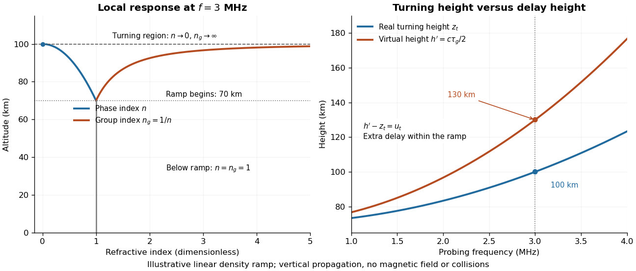
An original solvable profile makes the difference explicit. Approximate the region below by , and prescribe a linear rise of squared plasma frequency above it:Here the symbol denotes the penetration depth, and has units . In the propagating part of the ramp, . In the leading geometrical-ray delay model, with a frequency-independent turning connection wave phase, the round-trip group delay isThe endpoint singularity is integrable: substitute to obtain . This approximation does not resolve the finite-wavelength structure at the turning region. It illustrates the effect of slow group velocity before the return, rather than adding extra geometric altitude.
As an independent phase-based derivation, the propagation contribution to the round-trip wave phase isIts derivative agrees with the delay integral. Using the phase integral itself as a distance at speed would give instead of : wave phase, group delay and real turning height are three different quantities.
Choose and stipulate , where . ThenAt , the real turning height is but the virtual height is , corresponding to with . These stipulated parameters describe neither a measured profile nor a separate physical reflector at . Because the ramp has no density maximum, it also has no finite upper penetration threshold; a real bounded E layer or F layer requires a richer profile.

Partially filled coaxial capacitor Created 2026-10-18 Updated 2026-10-25
A long coaxial cylindrical capacitor of length and radii has a dielectric-filled overlap of length and relative permittivity . Neglecting end and interface fringing, its filled and vacuum portions are in parallel because both share the same two conductors. The electric potential difference produces in either portion; the electric displacement field and electrode charge differ by the local permittivity. Adding their capacitances gives the title formula. The dielectric boundary is axial while the interior electric field is radial and tangential to that interface, consistent with the electrostatic interface boundary conditions.
Toroidal sand dollar egg experiment 2026-10-18
In 1961, Raymond Rappaport gently removed membrane and jelly from sand dollar ova with a constricted pipette. After fertilization, he used an inverted optical microscope and rack-and-pinion manipulator to press a needle-mounted glass sphere through an egg onto the chamber floor, producing a torus-shaped biological cell. Visible spindle apparatus positions and cleavage furrow progression were the readout.[ref]
Experiments concerning the cleavage stimulus in sand dollar eggs by Raymond Rappaport. Experiments concerning the cleavage stimulus in sand dollar eggs, pp. 81–82, Materials and Methods: egg preparation, inverted microscope and sphere manipulation
First cytokinesis opened one side into a horseshoe containing two cell nuclei. During the next division, daughters separated from its free ends; an additional cleavage furrow crossed between mitotic asters of different spindle apparatuses. Control eggs supplied the timing comparison. This region lacked intervening chromosomes or a previous nearby spindle apparatus. This supported mitotic aster-associated positioning, without identifying the signal or establishing universal necessity.[ref]
Experiments concerning the cleavage stimulus in sand dollar eggs by Raymond Rappaport. pp. 81–82, introductory experiment summary, Results §1 and Figure 1 legend: horseshoe, second division, control comparison and furrowing between separate mitotic figures
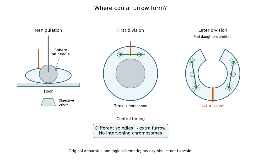
Manipulation and inference in the toroidal sand dollar egg experiment
. Original apparatus and logic schematic; mitotic aster rays are symbolic. Details.
Classical ideal gas in a spherical linear trap Created 2026-10-18 Updated 2026-11-05
For a structureless particle with Hamiltonian , , the classical phase space integral gives the displayed one-particle partition function. Its spatial integral is , while the momentum integral gives . For indistinguishable dilute particles, , , and . These thermodynamic formulas use leading Stirling accuracy; the classical phase-space integral additionally requires temperatures above the discrete trap level scale.
Circumference 2026-10-18
The circumference of a circle is its boundary arc length. For radius , it equals . This growing boundary length accounts for the radial factor in the Rayleigh distribution.
Circular sector 2026-10-18
A circular sector is the portion of a disc between two radii and the connecting circle arc. If its radius is and its central angle is radians, its area isIndeed, polar coordinates give . The full disc corresponds to , a semicircle to , and a quarter-disc to . In a solid with horizontal sector cross-sections, radius and angle , its volume is . Holding the angles and heights fixed while scaling every radius by a factor scales that volume by .
Circular arc Created 2026-10-18 Updated 2026-10-20
A circular arc is a connected portion of a circle. For radius and subtended central angle measured in radians, its arc length is . Two distinct endpoints determine two circular arcs: when they are not opposite, the minor arc has and the major arc has . Opposite endpoints determine two semicircles. The straight line segment joining the endpoints is a chord, rather than the curved circular arc itself.
Polarization CHSH count model Created 2026-10-18 Updated 2026-10-25
Let be orthogonal linear polarizations, and prepare the Bell state . The analyzer vector is ; its orthogonal companion has outcome . Direct inner products with the Bell state give and . Thus the expectation value of the outcome product is . These are physical polarizer angles; their corresponding Bloch sphere angles are doubled.
For a stipulated isotropic admixture, use the density matrixThe maximally mixed state contributes zero correlation, so for . Each local marginal is , independently of the other setting, illustrating quantum no-signalling. In this model is the interferometric visibility of the coincidence fringe; other noise models need not have one common visibility for every basis.
Choose , , and . The four correlations in the displayed CHSH inequality are . Consequently , exceeding the local bound exactly when . Perfect correlation at a single common setting would not yield this comparison between incompatible quantum measurements.
To connect probabilities with expected counts, stipulate emitted pairs per setting pair and independent detection efficiencies , independent also of settings, outcomes and hidden variables. The expected joint counts are . Their normalized correlation isFor original teaching inputs , , and , the expected counts are and . They total and give , hence . Fractional expected counts are not measured data. Efficiency cancels here because the loss model was specified to be independent; this algebra supplies no justification for discarding failures in an arbitrary Bell test with a detection loophole.
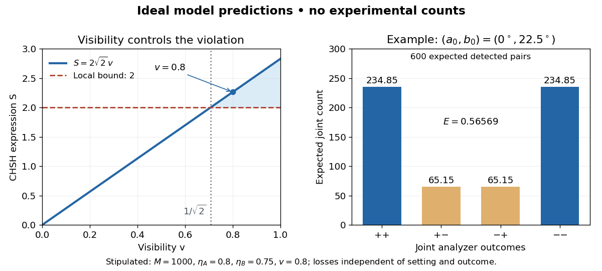
Ideal CHSH visibility threshold and expected detection counts
. Original model predictions, not experimental data. The first panel shows the visibility needed to exceed the local bound. The second uses 1000 emitted pairs, efficiencies 0.8 and 0.75, and visibility 0.8; each bar is an expected joint count. Details.
For the displayed metric tensor, its inverse has components and . The nonzero second-kind Christoffel symbols are , and . They follow by differentiating the two diagonal metric entries and raising the first index of the first-kind connection coefficients. Polar coordinates require treating separately.
Chemical equilibrium of a classical spin gas Created 2026-10-18 Updated 2026-11-05
For a nondegenerate spin-one-half ideal gas with energies , the two component chemical potentials are . Diffusive and spin-conversion equilibrium require one spatially constant common chemical potential, provided spin conversion is allowed. Hence the displayed densities give total number density and magnetization . The high-temperature fixed-density limit is , a Curie law. At fixed chemical potential the density itself varies with temperature, so the unnormalized magnetization need not have a pure dependence.
For noninteger real , expand a smooth forcing as in Chebyshev polynomials. Because , division of each coefficient by gives the regular solution. The coefficients use the weighted inner product with weight . Choosing the same endpoint domain as the regular eigenfunctions of the Sturm-Liouville problem is essential: finite values alone also allow homogeneous solutions and , which generally have divergent endpoint derivatives. Setting converts the regular endpoint condition into the Neumann boundary conditions . The homogeneous equation then has no nonzero solution when is noninteger, proving uniqueness in this domain.
For the Chebyshev differential equation , a power series about the ordinary point zero splits into even and odd solutions with the displayed recurrence relation. Every nonterminating parity series has radius of convergence one. If for a nonnegative integer , the parity series containing terminates, giving a polynomial with infinite radius of convergence; the other independent series still has radius one. Normalized solutions are and , with the latter replaced by when .
There are unlisted articles, also show them or only show them.