
For a nondegenerate parity-symmetric ground state in an external electric field, write the perturbation as . The first-order state correction givesThe positive coefficient is the electric polarizability along the applied direction. Meanwhile second-order nondegenerate perturbation theory gives . Thus the induced electric dipole moment satisfies , not . The Hellmann–Feynman theorem independently gives .
Dynamic electric polarizability Created 2026-10-18 Updated 2026-10-20
The dynamic electric polarizability relates the induced electric dipole moment at a driving frequency to the applied electric field at that frequency in linear response theory. A complex coefficient can encode both a dispersive phase and absorption. For a charged one-dimensional quantum harmonic oscillator with charge magnitude , mass , and natural frequency , the undamped response isOne derivation uses the oscillator electric-dipole selection rule and first-order time-dependent perturbation theory. The same result follows from the classical Lorentz oscillator model: and imply . At exact resonance there is no bounded periodic response without damping; a finite switch-on produces secular growth rather than a finite steady-state value of the pole expression.
Electric dipole field 2026-10-18
At distances large compared with the separation of a neutral charge pair, its electric field has the displayed leading form in terms of the electric dipole moment . Measure the polar angle from . The radial and angular components are and , giving . At fixed radius the polar field magnitude is twice the equatorial one. This leading neutral-pair field falls as , faster than the electric field of an isolated point charge.
Torsional waves in a solid circular rod Created 2026-10-18 Updated 2026-10-20
For small torsional displacement , the transmitted torque is . A slice of length receives net torque and has axial moment of inertia . Its angular equation therefore gives the displayed wave equation, with wave speed . The same geometric factor cancels from inertia and stiffness, making this ideal torsional speed independent of rod radius. This long-wave circular-rod model neglects additional elastic modes and dissipation.
Coherent elastic scattering Created 2026-10-18 Updated 2026-10-20
In coherent elastic scattering, amplitudes from the scattering constituents combine while their internal state is unchanged. For X-rays, recoil taken by a whole chemical atom can produce an effectively unshifted component alongside the Compton scattering component.
Maximum laboratory deflection in relativistic elastic scattering Created 2026-10-18 Updated 2026-10-20
A projectile of mass elastically scattering from a stationary target of mass has the displayed maximum laboratory angle. In units, let its incident energy be and . Boosting the outgoing four-momentum from the center-of-momentum frame gives , with and . The maximum at has . Equality is allowed; a strict upper bound would exclude a realizable outgoing direction. The angular cap is independent of incident energy.
Calibrated Einstein-de Haas torsion response 2026-10-18
An original reduced model makes the calibration explicit. Let the torsion pendulum have restoring torque , with torsion constant , and viscous damping torque , with . Allow an unwanted axial torque :Here is the undamped natural angular frequency and the quality factor. The forced harmonic oscillator response must be included before a twist can be interpreted as a torque.
Using the complex amplitude convention and similarly for and , differentiation multiplies by . Substitution givesThis is the torque-to-twist transfer function. With and real positive , the twist amplitude isFor , the twist phase relative to is . At it is zero, although the reaction torque leads by . A phase measured at the mirror is not automatically the phase of the applied torque.
A fixed-amplitude reference torque measures directly. The Einstein-de Haas effect instead contains an extra factor when stays fixed. Consequently its twist amplitude peaks exactly at in this model, whereas the fixed-torque peak is at when . To verify the first statement, divide the squared denominator of by : the quantity to minimize is , minimized at . Both response curves tend to zero at high frequency; only the magnetomechanical curve also tends to zero at zero frequency.
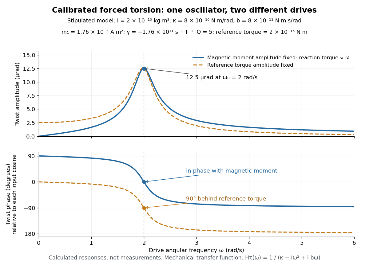
Calibrated forced torsion: distinguish the mechanical response from the magnetic drive
. Original calculated curves, not historical measurements or fitted data. A constant reference torque and a constant-amplitude magnetic dipole moment share the same mechanical transfer function. The lower plot uses each input's own cosine as its phase reference. Markers at show equal twist amplitudes but different phases. Details.
For a fully stipulated example, choose , , , , and . These teaching inputs give , , reaction torque amplitude at , andAn optical lever at distance gives small-displacement spot amplitude ; its full peak-to-peak width is . For a fast reversal from to , the same inputs give and initial , provided the external angular impulse is negligible.
One independent mechanical calibration adds known moment of inertia , keeping unchanged. If are the undamped oscillation periods before and after adding it, thenFor in the stipulated example, and , recovering the chosen and . Real damped periods require a damping correction: a free decay has angular envelope and oscillation angular frequency . Measuring that decay determines . Calibrating the optical scale, mechanical response and change of magnetic dipole moment separately is what makes the inferred gyromagnetic ratio meaningful.
Einstein-de Haas experiment 2026-10-18
In 1915, Albert Einstein and Wander Johannes de Haas suspended a soft-iron cylinder by glass fibre between coaxial coils. Alternating magnetization drove torsional resonance; a mirror reflected lamplight onto a scale. They compensated Earth's magnetic field, tilted the coils, and rotated the suspension attachment to test unwanted magnetic dipole torques. Added known moment of inertia calibrated the mechanical response.[ref]
Experimental proof of the existence of Ampère's molecular currents by Albert Einstein and Wander Johannes de Haas. §§4–5, pp. 702–706: apparatus, controls, calibration
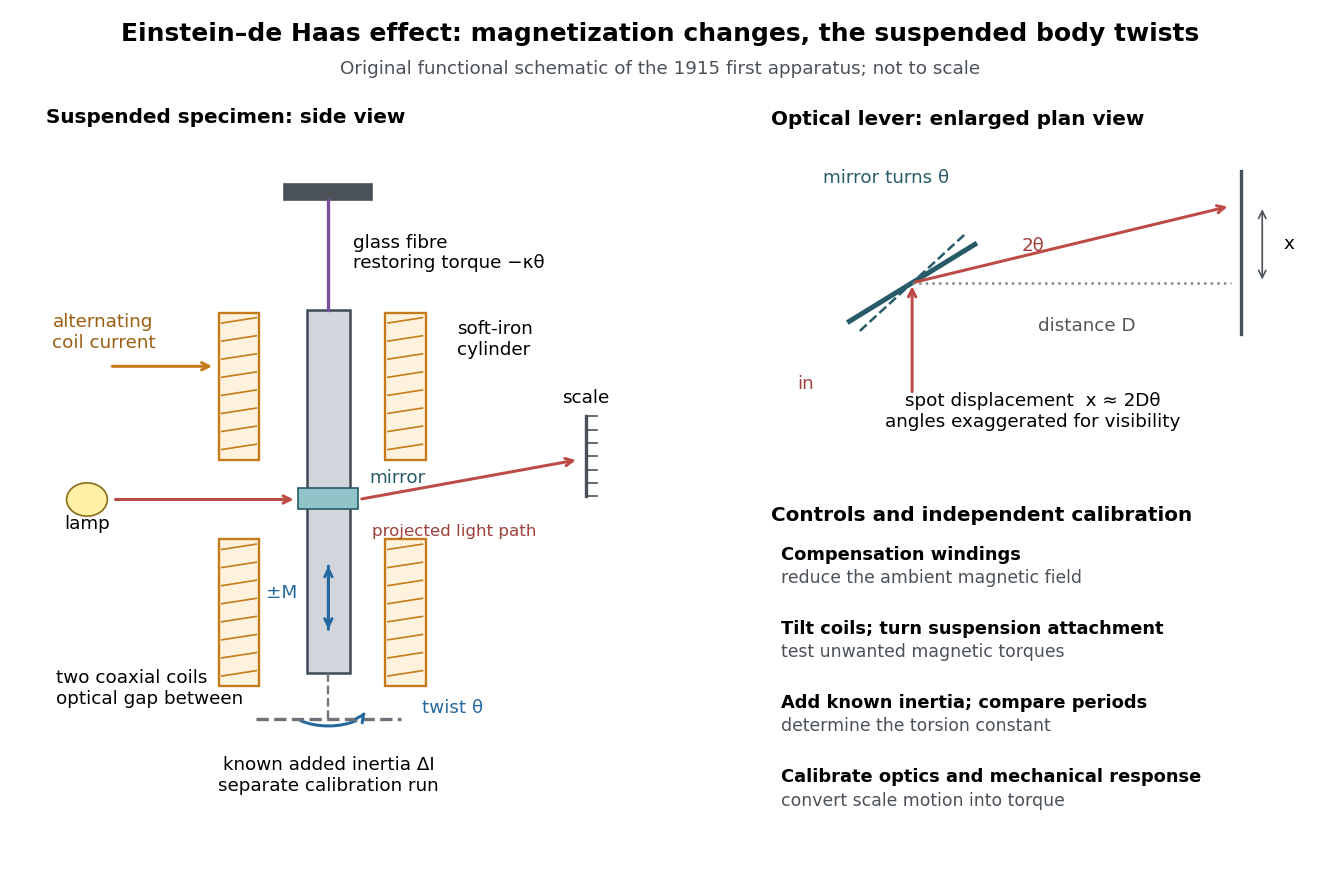
Einstein-de Haas experiment: suspended magnet, drive and optical readout
. Original functional schematic of the first apparatus, rather than a scale reconstruction. The split coaxial coils leave an optical gap. The enlarged plan view explains the optical lever; the calibration bar is attached for a separate calibration run. Compensation windings are represented by their function. Details.
Their paper acknowledges a failed phase determination and claims only ten-percent precision for the revised measurement. Its agreement with the orbital gyromagnetic ratio prediction was not a direct discovery of spin.[ref]
Experimental proof of the existence of Ampère's molecular currents by Albert Einstein and Wander Johannes de Haas. §6, pp. 706–707: phase failure; §7, pp. 707–711: resonance, precision
Comparing that orbital gyromagnetic ratio prediction with the electron spin g-factor explains why a successful qualitative demonstration of angular momentum transfer can coexist with an inadequate quantitative interpretation. The stated precision is the authors' estimate; it does not establish that all systematic errors were bounded by that amount.The general control problem follows directly from the model. Unwanted magnetic dipole torque can drive the same mechanical resonance as the desired reaction torque. In the ideal geometry and alone produce no axial cross product, but transverse magnetic dipole moments, stray transverse magnetic fields and imperfect alignment can. Nulling stray magnetic fields and deliberately varying alignment test this contribution. Merely observing a large resonant twist cannot identify its cause.
For a nearly instantaneous magnetic response, a sinusoidal magnetization makes follow the drive while is in phase quadrature. An ordinary magnetic contribution proportional to is then distinguishable by phase, after removing the mechanical frequency response. Hysteresis or delayed magnetic response can spoil this simple separation. The measured magnetization, rather than the coil electric current alone, must set the reference. Mechanical vibration, magnetostriction coupled through imperfect geometry, and changing suspension properties require separate checks; none is eliminated simply by reversing the coil electric current.
Magnetomechanical angular momentum balance Created 2026-10-18 Updated 2026-10-20
Let be the axial magnetic dipole moment, where is the axial magnetization. Write for the internal angular momentum associated with that magnetic dipole moment, and for the body's rotational angular momentum, with moment of inertia . In a regime admitting a constant signed gyromagnetic ratio , axial conservation of angular momentum givesHere names the internal reaction torque on the body, not an additional external torque. The external term includes the suspension. The model assumes that the changing internal angular momentum is transferred to the measured mechanical motion, with other storage or escape channels negligible on the observation timescale. A changing or non-collinear mixture of orbital angular momentum and spin angular momentum need not admit a single constant .
During a reversal fast compared with the mechanical response, with negligible external angular impulse, integrating the balance givesFor and an electronic , the body acquires : its initial rotation is toward by the right-hand rule. Reversing the reversal reverses the impulse. Over a complete periodic cycle, , so the net reaction angular impulse vanishes; a resonant alternating response does not imply steadily accumulating angular momentum.
The orbital angular momentum prediction can be derived without a material model. A charge traveling around a circle of radius at angular frequency has loop electric current and magnetic dipole moment . Its orbital angular momentum is , hence, for an electron with electric charge ,The electron magnetic moment associated with intrinsic spin instead obeysHere is the elementary charge, is the electron mass, and is the electron spin g-factor.[ref]
The magnetic moment of the electron by Polykarp Kusch. pp. 299–300: orbital and intrinsic moments and the Dirac value
Thus the same change of magnetic dipole moment corresponds to about half as much transferred angular momentum in the pure-spin model as in the orbital angular momentum model. This factor of two is a relation between magnetic dipole moment and angular momentum, not evidence that an electron is literally a rotating charged sphere. In a material with both contributions, the inferred coefficient is a material-dependent magnetomechanical gyromagnetic ratio. Odd-dimensional real matrix with positive determinant has a positive eigenvalue Created 2026-10-18 Updated 2026-10-25
For a real square matrix of odd size, if , then has a positive real eigenvalue. Its characteristic polynomial is monic of odd degree, so and as . The intermediate value theorem supplies a positive root. This proves the claim without assuming that all eigenvalues are real. The odd-size hypothesis is essential: in even dimension has positive determinant and only the negative eigenvalue .
Earth's rotation Created 2026-10-18 Updated 2026-10-20
Earth's axial rotation relative to an inertial frame. The Foucault pendulum detects its component along the local vertical through the Latitude law of Foucault precession.
Double-slit interference Created 2026-10-18 Updated 2026-10-20
Double-slit interference depends on the relative wave phase and first-order optical coherence of two collected fields. For equal separately measured intensities, the interferometric visibility is . A small source direction change introduces phase difference for projected interferometric baseline .
An algebraic simplification proves equality only where both original and transformed expressions are defined. If a cancelled factor vanishes at a point, the simplified expression may instead describe an extension to that point. For example,holds only when and . The right side is zero at , but the left side is undefined there. A graph of the original function must retain those holes. The extension may be useful, but it is a different function with a larger domain of a function.
Dirichlet eigensystem of a rectangle 2026-10-18
On , with positive side lengths and zero Dirichlet boundary conditions, separation of variables for giveswith the displayed eigenvalues. The one-dimensional endpoint conditions exclude constant and hyperbolic factors and force the positive integer sine frequencies. The product Fourier sine series basis is complete in the square-integrable functions on the rectangle. Consequently an eigenfunction with prescribed is a linear combination of exactly those modes with ; if none match, only the zero solution exists. Distinct pairs with the same sum give an eigenvalue with geometric multiplicity greater than one. On a square of side , for instance, has precisely the pairs and , so its eigenspace has dimension two.
For , the decaying solution of on the positive half-line with follows by integrating the Dirichlet half-line Green function for minus d2 plus 1:Both and are continuous at , whereas has the jump required by the bounded step in the forcing. Its common value there is .
Dirichlet Green function inside a hemisphere 2026-10-18
For the upper half of a three-dimensional ball, let be the reflection of an interior source in the equatorial plane. The Dirichlet Green function inside a sphere, evaluated at the source and its reflection and then subtracted, vanishes on both the spherical cap and flat equatorial disc. Reflection makes the source distances and image distances agree on the plane. Only the original source is in the upper half-ball; the reflected source is in the lower half-ball, and both inversion images are outside the ball. Thus the difference has precisely the required Dirac delta distribution and Dirichlet boundary conditions.
Dirac Hamiltonian Created 2026-10-18 Updated 2026-11-05
The Dirac Hamiltonian is the first-order time-evolution operator obtained from the Dirac equation. For a free massive particle,where the Dirac matrices satisfy , and . These identities give , recovering the relativistic energy-momentum relation.
Minimal electromagnetic coupling replaces the canonical momentum by and adds , in SI units. The wavefunction has spinor components, and the free operator has positive- and negative-energy branches. The Dirac field interprets particle and antiparticle excitations with a stable vacuum; it is more complete than treating the negative branch as an ordinary one-particle spectrum with no lower bound.
For constant on all space and time, the active waveform transformation leaves the action of invariant: the density gains and the integration measure gains . With canonical momentum , its Noether current can be chosen asThe integrated charge is conserved if its boundary flux vanishes and the weighted integral exists. For a rightgoing wave packet , , it becomes . A fixed finite interval generally breaks this scale symmetry unless its boundaries and boundary data are transformed too.
Scale-breaking sources in derivative field theories Created 2026-10-18 Updated 2026-11-05
For a first-derivative real scalar field in one space and one time dimension, put . Its on-shell divergence isA quadratic derivative density with arbitrary field-dependent coefficients has zero derivative-homogeneity term. An extra term instead gives . A position-dependent kinetic coefficient gives . These source terms distinguish scale invariance from internal field-shift symmetry.
Conjugacy classes of a finite dihedral group Created 2026-10-18 Updated 2026-10-20
Use for the group of order with rotation and reflection . Every element is or , . The rotational conjugacy classes are the sets , reduced to singletons for central rotations. For odd , all reflections form one class, giving classes in total. For even , the identity and are central singletons, the other rotations form pairs, and the reflections split into even and odd powers of , giving classes. Indeed conjugation by changes a reflection exponent by , while conjugation by negates it. For odd prime , a normal subgroup containing a reflection must contain all reflections and hence the whole group; the proper normal subgroups are therefore only the identity subgroup and the rotation subgroup.
There are unlisted articles, also show them or only show them.