
Dirichlet eigenfunctions of the Chebyshev differential operator Created 2026-10-18 Updated 2026-10-20
The Chebyshev differential equation on , with zero endpoint values, has the Sturm-Liouville formThus and the weight defining the weighted inner product is . The substitution maps the problem to on with homogeneous Dirichlet boundary conditions. It also transforms into . Consequently the normalized eigenfunctions areTheir weighted inner product is the ordinary sine inner product on . Equivalently, , where is a Chebyshev polynomial of the second kind. These are not the cosine solutions , which have different endpoint values. The original endpoints are singular because vanishes and diverges there, but the transformed Dirichlet problem specifies the self-adjoint realization. The eigenfunctions vanish at both endpoints and their quasi-derivatives have finite limits, so the boundary form vanishes.
Work by Charles M. Stein 2026-10-18
Early CCD charge-transfer experiment 2026-10-18
George Elwood Smith reports fabricating MOS capacitors, thermally generating the first packet, and clocking it to an output that pushed it into the substrate for electric current detection. A later integrated eight-bit device demonstrated imaging. Dark or reversed-clock control traces are not specified; feasibility alone does not calibrate charge-transfer efficiency.[ref]
Nobel Lecture: The invention and early history of the CCD by George Elwood Smith. pp. 2309–2310, Figs. 7–9, prototype and imager
A discriminating repeat would compare identical cycles with and without initial carrier injection, then suppress or reverse the transfer sequence while retaining output switching. An electric current transient synchronized with gate switching can include capacitor feedthrough; only the difference tied to initial electric charge and the expected transfer delay tests packet transport. These are proposed controls, not controls documented in the lecture. For an optical version, a blocked exposure estimates dark current and read noise; a spatially isolated illuminated optical detector pixel exposes any deferred charge in CCD readout trail. Photon shot noise persists even with ideal transfer.
Deferred charge in CCD readout Created 2026-10-18 Updated 2026-10-20
Deferred charge in CCD readout reaches later output samples than its originating packet. George Elwood Smith describes surface states at the silicon–silicon dioxide interface capturing electrons and releasing them later, smearing the image. A buried channel keeps the stored packet away from that interface.[ref]
Nobel Lecture: The invention and early history of the CCD by George Elwood Smith. pp. 2310–2311, Figs. 10–11, trapping
An original comparison separates two interpretations of the same main-packet deficit. If a single transfer defers fraction by exactly one sample and loses nothing, an isolated input packet produces samples followed by : summing both recovers . A truly lossy transfer yields only , with no later recovery. For and , both give in the intended sample, but only the deferred case gives a -electron trail. Such a trail redistributes position information even when total electric charge is conserved. Repeated delays require a time-response model; alone cannot predict trail shape. Electron-hole recombination, escape to another contact, or release beyond the recorded window can instead remove signal from the measured sum.
Charge-transfer efficiency Created 2026-10-18 Updated 2026-10-20
The charge-transfer efficiency is the fraction of a packet delivered into its intended next site or time slot in one transfer, under stated conditions. It is distinct from quantum efficiency, which concerns conversion of incident photons into collected charge carriers. Define the complementary inefficiency as .
In an original model with constant , let denote the mean number of original packet electrons still delivered on time after transfers. Assuming no reinjection into that packet,Repeated substitution proves the result; for different efficiencies the fraction is . For , a Taylor expansion of gives , while the simpler requires .
Choose and . For , the expected on-time output is electrons; for , it is . These are model means, so fractional electron counts do not describe an individual packet. Even a small per-transfer imperfection can imprint distance-dependent image errors.
If every original electron independently stays on time with probability , a fixed initial count gives a binomial distribution with variance . An initial Poisson distribution with mean instead gives an on-time Poisson distribution with mean and variance , by Poisson thinning. A deterministic attenuation formula alone does not specify noise. Real trapping can correlate packets and depends on timing, illumination and temperature; the independent constant-efficiency model then fails.
CCD clocked charge transfer Created 2026-10-18 Updated 2026-10-20
For an electron packet, a sufficiently positive gate electric potential attracts electrons beneath the insulating layer of a MOS capacitor. The corresponding potential energy is , where is the magnitude of elementary charge: a larger electric potential gives a deeper potential well for electrons. A drawing of potential energy must therefore reverse the vertical sense of a drawing of electric potential.
A simplified three-phase transfer raises the adjacent gate's electric potential before lowering the old holding gate. This overlaps the accessible regions, then leaves the packet under the new gate. Repeat with the next gate to move it forward. Isolated wells with an intervening barrier would store the packet without transferring it.[ref]
Charge Coupled Semiconductor Devices by Willard Sterling Boyle and George Elwood Smith. Boyle and Smith, 1970, p. 587, neighboring capacitors and manipulated electrode potentials
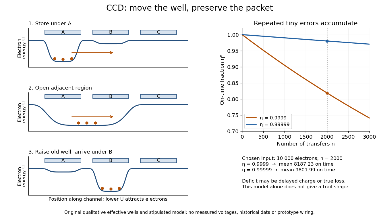
CCD clocked charge transfer and cumulative charge-transfer efficiency
. Original explanatory potential energy profiles show storage, overlap and arrival, with lower curves meaning more attractive regions for electrons. These are qualitative effective profiles, not measured voltages or prototype wiring. The right panel calculates the main-packet fraction for the stipulated constant-efficiency model; charge absent from that packet may be deferred or truly lost. Details.
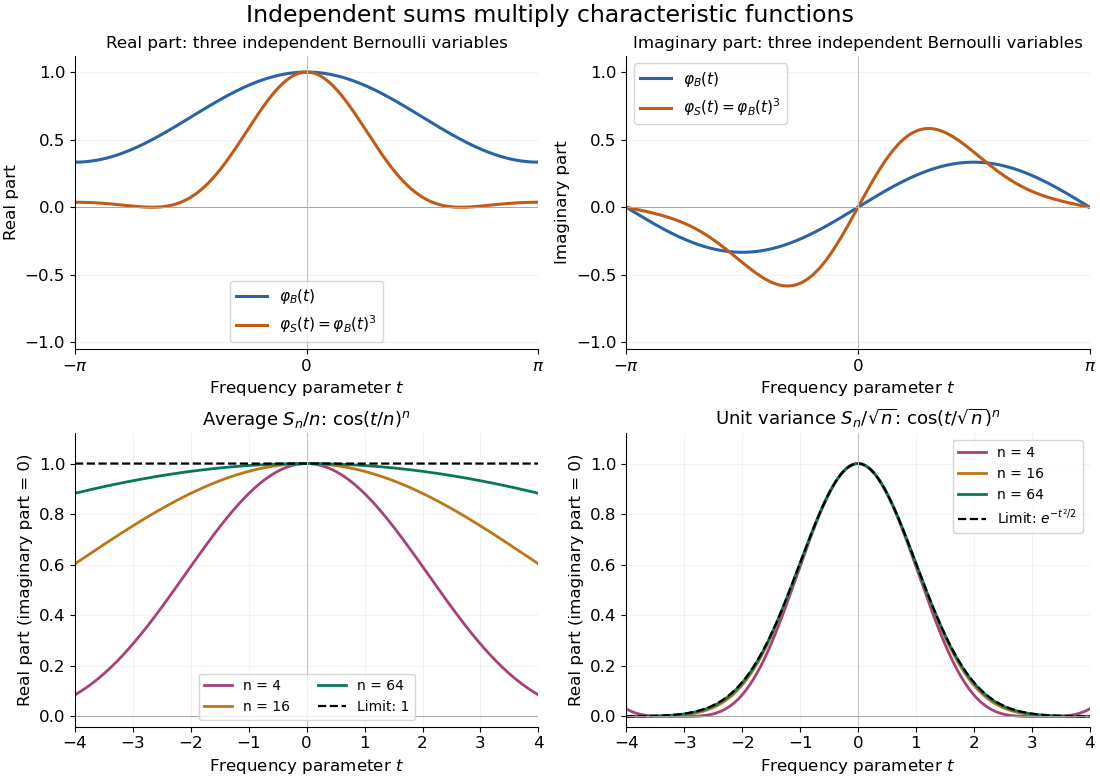
Let be independent and identically distributed random variables taking and with equal probabilities, the Rademacher distribution. The two opposite complex exponentials give . Their expected value is zero and their variance is one. For , the characteristic functions of its sample mean and its variance normalization are respectivelyFor each fixed , the bases are positive for all sufficiently large . The Taylor expansion at zero then givesExponentiating proves the two displayed pointwise limits. The first limit is the characteristic function of the constant zero; the second is that of the standard normal distribution. The Lévy continuity theorem gives the corresponding convergence in distribution statements. Averaging has variance , whereas dividing the sum by preserves variance one. This sign calculation illustrates why the law of large numbers and the central limit theorem use different scales; it is not a proof for arbitrary probability distributions.
Let be independent random variables, each with the Bernoulli distribution of parameter , and let . Multiplying their characteristic functions and expanding by the binomial theorem givesThe coefficients are exactly the probability mass function of the binomial distribution with parameters : the sum takes with probabilities . Direct outcome counting verifies them: an outcome with ones has probability , and there are such outcomes. The coefficients sum to one, recovering .
At , . This is also : the complex exponential now records parity. The moments agree by two routes: linearity of expectation gives , while the variance of a sum of independent random variables gives . Summing gives the second moment , also recovered as .

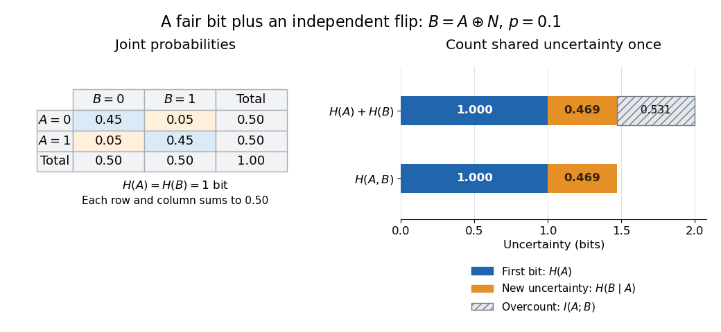
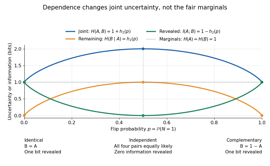
Correlated binary variables 2026-10-18


Inverse Cayley transform of a unitary matrix without eigenvalue one Created 2026-10-18 Updated 2026-11-05
If is a unitary matrix with no eigenvalue equal to one, the displayed inverse Cayley transform of a Hermitian matrix is Hermitian. Since , taking the Hermitian conjugate gives , using commutativity of rational functions of . An eigenvalue is mapped to the real number . Conversely , so this correspondence identifies Hermitian matrices with unitary matrices whose spectrum avoids one.
Dispersive atom-cavity coupling Created 2026-10-18 Updated 2026-11-05
Dispersive atom-cavity coupling is the off-resonant regime where real excitation exchange is suppressed but virtual mixing shifts the energies. For a two-level system describing an chemical atom coupled to one mode, the scale appears when is large compared with the relevant occupation-enhanced coupling .
An effective term proportional to then makes the atomic phase depend on photon number and the cavity frequency depend on atomic state. Measuring that phase can infer field occupation without resonantly absorbing a photon in the ideal approximation. Finite detuning, losses and probe backaction still matter; dispersive does not mean completely uncoupled or universally disturbance-free. A model must state detuning sign and the retained perturbative order.
Tangent of a uniform angle has a Cauchy distribution Created 2026-10-18 Updated 2026-10-20
If and has the continuous uniform distribution on , then has the Cauchy distribution with location zero and scale . The tangent function is strictly increasing on this interval, so its cumulative distribution function isDifferentiating gives the probability density function . The probability of either endpoint is zero, so including endpoints in the uniform interval does not alter this probability distribution. The slow quadratic decay makes the expected value undefined: its positive and negative parts both have infinite integrals. Its second moment is also infinite, so it has no finite standard deviation.
For speed in , Fermat principle gives the elapsed-time integrand . Its symmetric stationary light rays through are the displayed catenaries. Set . The endpoint equation is . This function decreases and then increases, with unique minimum where . Thus above the minimum there are two stationary rays, at the minimum one, and below it none. The travel time on either ray is , and its minimum height is .
For and , one solution is , with . A second has , with . Hence these endpoints do not uniquely specify the ray. Stationarity is distinct from global minimization: paths descending almost to have limiting travel time , below either stationary value in this example.
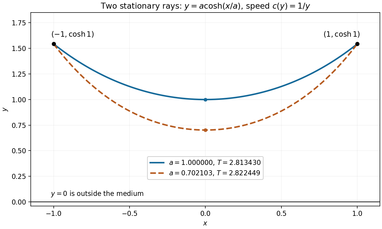
Two stationary catenary rays connect the same endpoints
. For speed , the endpoints and admit stationary light rays with minimum heights and . Their different travel times illustrate that Fermat principle is a stationarity condition. Details.
Given injections and , start with the set difference : these are exactly the inputs for which is unavailable. Follow both functions repeatedly, using the natural-number recursion theorem to defineThus contains all the members reachable from any starting point in . The notation and denotes images of a function. If is the empty set, then every is empty and alone gives the desired bijection.
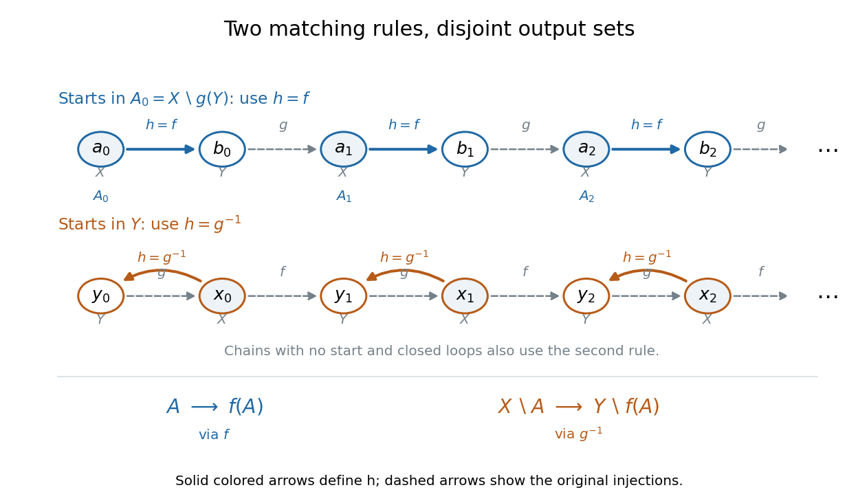
The Injection-chain proof of the Cantor-Schröder-Bernstein theorem partitions the inputs into two matching rules
. The upper row shows a chain seeded in , where the bijection follows . The lower row shows a chain beginning in , where the bijection reverses . The same rule also handles chains with no starting point and closed loops. Separate and copies are used even if the original sets overlap. Details.
Define a function on all of byHere is the inverse function from to , obtained by restricting the codomain of to its image. It is well defined because is injective. Every belongs to , since , so the second rule is always available where it is used.
The decisive set identity isThe last equality holds because every with lies in , whereas is disjoint from . Consequently, for any ,Indeed, cannot belong to ; if it lies in , the identity gives for some , and injectivity gives . The converse follows directly by applying .
Now restricts to a bijection from onto . The displayed equivalence says that restricts to a bijection from onto , so its inverse function bijects the remaining inputs with the remaining outputs. The two input sets partition and the two output sets partition . Their combined function is therefore both injective and surjective.
No choice function is needed: is fixed by the given injections, and each required is unique. We neither choose a representative from each chain nor enumerate . This is a proof in ordinary classical ZF, even when no well-ordering of the sets exists there.[ref]
Cantor-Schroeder-Bernstein Theorem by Paul Garrett. Paul Garrett, Cantor-Schroeder-Bernstein Theorem, pp. 1–2, chain construction and pairings; p. 1, no invocation of the axiom of choice
Take , the nonnegative integers, and , the positive integers. Choose the injectionsHere is an inclusion map, while reaches only the positive even integers. In particular, is not a bijection: it misses every positive odd integer. Simply using the inverse function of on its image misses input zero.
The remedy is to follow the alternating injections starting at the missing input zero:The subscripts distinguish an input in from an output in , even when their numerical values agree. The resulting subset of is . Its sequence of members satisfies and , giving by mathematical induction. Define the function
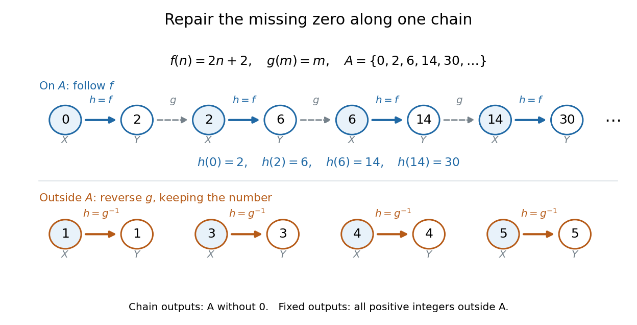

The image covers all the positive members of exactly once. The other inputs cover exactly once by staying fixed. These output sets are disjoint and their union is , proving that is a bijection. In particular, , , , while and .
For completeness, its inverse function isThe familiar bijection also works, but this example shows something more specific: the two chosen injections can repair the missing zero by moving only a sparse sequence of inputs. The repair never has to shift the entire set.
BABAR time-dependent CP violation experiment Created 2026-10-18 Updated 2026-10-20
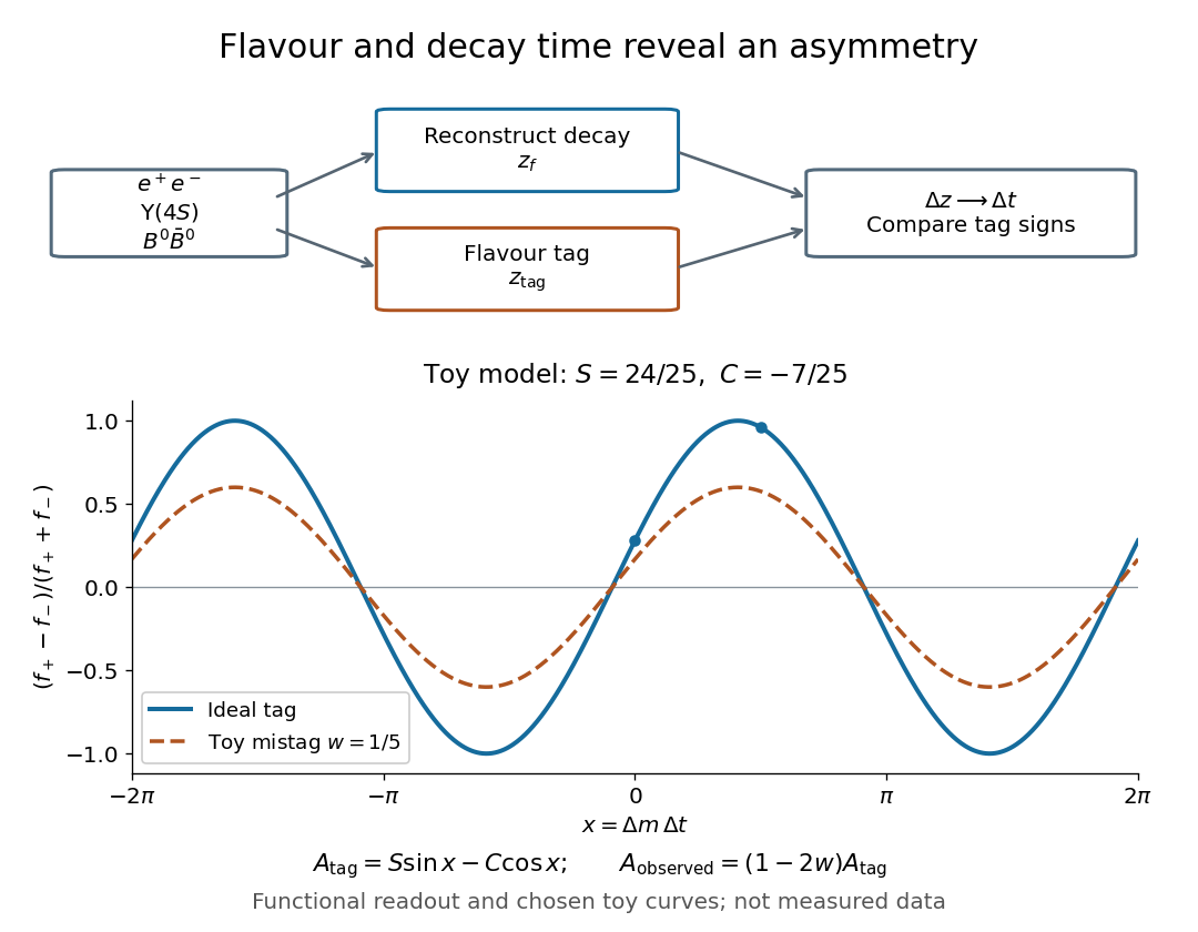
BABAR used asymmetric electron-Positron collisions near the Upsilon meson resonance to prepare neutral B meson pairs. It reconstructed one decay into charmonium plus a kaon, and used flavour tagging on the other B meson with charged leptons or kaons. Silicon tracking reconstructed decay vertices for the decay-time difference. Self-tagging decays calibrated mistags and time resolution; charged decays provided a control. The tagged time distributions established CP violation, limited by backgrounds, mistags and vertex alignment.[ref]
The Lorentz boost converts vertex separation to at leading order. Unequal beam energies thus make a time difference measurable as a distance.[ref]

Adiabatic buoyancy frequency of an ideal gas Created 2026-10-18 Updated 2026-10-20
For a gas of fixed composition in hydrostatic equilibrium, with upward and downward gravitational acceleration of magnitude , an adiabatic process gives the displaced element density change . Comparing with the ambient change yieldsThe ideal gas law and give the title expression, where is the constant-pressure specific heat capacity. A temperature gradient less negative than the adiabatic lapse rate gives positive ; a steeper decline gives convective instability.
Perrin sedimentation experiment Created 2026-10-18 Updated 2026-10-20
A colloidal grain in a liquid is large enough to see with a microscope, yet small enough for thermal motion to compete with its tendency to settle. In the Perrin sedimentation experiment, the equilibrium number density falls with height: a visible miniature atmosphere. Counting grains at different heights measures an energy scale; tracking their Brownian motion measures a transport rate. Connecting both to the same Avogadro constant makes the experiment a quantitative test of kinetic theory. The Wiener measure describes an idealized path law; these measurements instead test a physical model and its material parameters.
Jean Baptiste Perrin's 1909 memoir traces his sedimentation experiments to May 1908. It reports relative counts , , , at heights , , , , and compares radius estimates from Stokes settling velocity, counted grain mass, and rows of touching grains.[ref]
Mouvement brownien et réalité moléculaire by Jean Baptiste Perrin. 1909 memoir, §§15, 20–22; scan pp. 28, 41–49
The 1926 lecture describes resin precipitated from alcohol into water, washed and fractionated by centrifugation to obtain nearly monodisperse gamboge or mastic grains. Diameter and density were measured separately. A sealed slide-and-cover-glass chamber prevented evaporation; a vertical microscope resolved roughly layers through a roughly depth. Refocusing and photographing compared layer populations after equilibrium; changing temperature reversibly changed the distribution.[ref]
Discontinuous Structure of Matter by Jean Baptiste Perrin. Nobel Lectures, Physics 1922–1941; Discontinuous structure of matter, 11 December 1926, pp. 148–150
In Les Atomes (1913), Jean Baptiste Perrin restricts the eyepiece view to fewer than five or six grains and alternates observations between heights. Focus displacement requires a refractive index correction to recover actual layer separation. Horizontal positions were marked with a camera lucida, usually every , and distances calibrated with a micrometer; the polygon joins sampled positions rather than recording the intervening trajectory.[ref]
https://fr.wikisource.org/wiki/Les_Atomes/III. Les Atomes, chapter III, §§61–64
[ref]https://fr.wikisource.org/wiki/Les_Atomes/IV. Les Atomes, chapter IV, §§70–75
Work by Bradley Efron 2026-10-18
Photon-recoil lag correlation Created 2026-10-18 Updated 2026-10-20
A photon-recoil lag correlation asks how often a photon record occurs at a specified time displacement from an electron record. Let be observed separate-channel rates, the rate of detected genuine pairs before a timing cut, and their normalized timing probability density function. For an original dilute, stationary model with observation time , neglecting end effects and detector dead time, the expected pair density isThis counts all pairs of records, rather than at most one detector trigger per electron. It uses independent unrelated detections for the flat term and an added same-event contribution. A normal distribution for timing spread is a chosen approximation, not a claim about the historical instrument. Intrinsic emission delay, counter response and readout uncertainty can all affect the observed probability density function.
Define the accepted lag interval by : is its full width. Integrating the flat baseline gives the existing accidental coincidence expectation . The additional area is . Moving a window of the same full width away from the peak tests the baseline under the model's stationarity assumption. It does not remove correlated instrumental backgrounds or changing rates automatically.
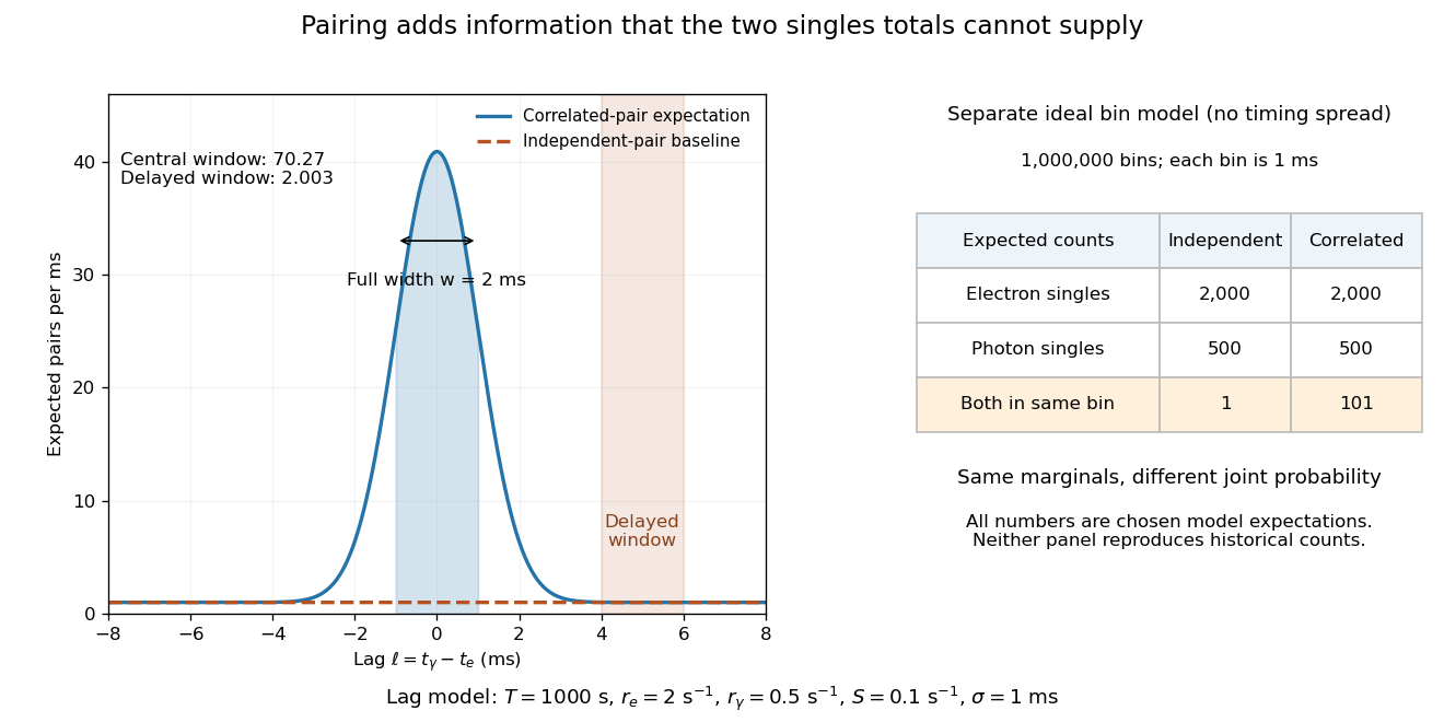
Lag-dependent pairs and a joint probability distribution carry information absent from singles totals
. Original chosen models, not historical counts or fitted data. Left: a normalized normal distribution of genuine-pair lags with standard deviation is added to an independent-pair baseline. Shaded intervals have full width , centered at zero and . Right: a separate exact ideal-bin model ignores timing spread; the two populations have identical singles expectations but different joint expectations. Details.
For the lag model, choose , , , and timing standard deviation . A full width gives expected accidental coincidences and accepted genuine pairs, using the error function. The total is approximately , whereas the displaced interval from to has approximately expected pairs. A finite sample fluctuates around these expectations; these values are not measured counts or a significance calculation.
The right panel isolates the information lost by retaining singles totals alone. In a separate idealized model, stipulate independent bins, with Bernoulli distribution indicators for electron and photon detection in a bin. Set and . Independence predicts , hence one expected double detection. Alternatively chooseThese nonnegative probabilities sum to one and preserve both marginal probabilities, yet predict double detections in expectation. Their covariance is . This is an exact joint probability distribution illustrating pairing; it does not model the timing spread in the left panel or reconstruct either historical hypothesis quantitatively. Its lesson is why two singles totals cannot decide whether the observed events share a cause.
There are unlisted articles, also show them or only show them.