
Thermal noise measurement 2026-10-18
MIT's laboratory guide mounts resistors on an aluminum box beneath a metal beaker shield, with short twisted leads. Its SR560 amplifier uses nominal gain before a Krohn-Hite – band-pass filter; an oscilloscope reads root mean square voltage. Calibration sweeps an attenuated sinusoid and measures the actual gain . Students alternate the resistor and a short circuit, subtracting squared readings , and disconnect the ohmmeter during noise acquisition. Lead and input capacitance enter the gain-squared integral. With settings unchanged, varying electrical resistance or temperature tests the predicted mean square. The guide prescribes repeated readings and warns against averaging noise waveforms to zero. This is a documented teaching protocol, not a supplied dataset of measured outcomes.[ref]
Johnson Noise and Shot Noise: The Determination of the Boltzmann Constant, Absolute Zero Temperature and the Charge of the Electron by MIT Department of Physics. MIT Department of Physics, Johnson Noise and Shot Noise, pp. 5–9: equation (13), apparatus §III, calibration §IV.1, Figure 5, and shorted-input subtraction equation (20)
The subtraction requires care: shorting the input changes the source electrical impedance. An amplifier's input current noise can therefore produce different voltage noise in the two configurations; a shorted baseline alone does not remove that contribution. Gain drift, interference and insufficient observation time also limit the inference. These are limitations of interpreting the measurement, not corrections that can be inferred from the nominal signal bandwidth alone. In an independent analysis one would compare the measured difference withwhere represents the measured shunt capacitance and excludes that separately modeled shunt. If calibration already includes the same shunt response, applying the denominator again counts the attenuation twice. The thermal noise worked example and both original figures illustrate ideal models; they claim no measured agreement or measured value of the Boltzmann constant.
Resistor-capacitor equilibrium noise 2026-10-18
Connect one physical resistor across an ideal lossless capacitor , with no applied source and an ideal readout that draws no electric current. Represent the resistor by its noisy Thévenin equivalent. The resulting RC low-pass frequency response gives the stationary capacitor voltage power spectral densityIts mean square follows by the effective noise bandwidth calculation:This is also the equipartition theorem: the mean capacitor energy is . Raising makes the low-frequency spectrum taller and its width narrower in exactly compensating proportions. It changes the equilibration time , not the final variance.
The integral to infinity belongs to the ideal classical model. For a physical electrical circuit, assume thermal equilibrium, linear components with negligible extra dissipation, and a corner far below the frequencies where parasitic effects, frequency-dependent electrical resistance, or invalidate the model; the omitted high-frequency tail must be negligible. A finite-bandwidth instrument measures only part of this variance. Its input capacitance contributes to the total , and its finite input electrical resistance introduces both loading and its own thermal electrical noise.
For and , the predicted equilibrium variance is and the root mean square voltage is . At , and . At , and ; the equilibrium root mean square voltage is identical.
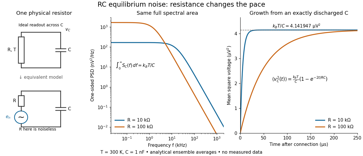

To obtain the growth curve, prepare exactly and connect the resistor at while maintaining its temperature. The RC low-pass filter's causal impulse response is for . Classical ideal white noise with two-sided power spectral density givesThe factor here is the two-sided time-domain noise intensity; the equilibrium spectral integral above used the one-sided . They give the same long-time limit. The variance approaches equilibrium with time constant , although a deterministic initial voltage decays with time constant . If the capacitor already starts in thermal equilibrium, its initial variance supplies the missing exponentially decaying term and the total variance stays constant.
Thermal noise worked example 2026-10-18
For an original hypothetical calculation, stipulate , , and an ideal rectangular measurement signal bandwidth . Using givesA matched electrical load receives root mean square from the source resistor, giving . These are stipulated model predictions, not laboratory measurements. Increasing raises the open-circuit voltage noise but does not increase the matched available power. Restricting the measurement signal bandwidth reduces root mean square noise as its square root; it improves signal-to-noise ratio only if the desired signal is preserved.
Thermal noise loading 2026-10-18
An external electrical load changes the terminal noise. Connecting a purely resistive load to the noisy resistor gives the voltage divider ratio . The source resistor's contribution at the load isIn a rectangular signal bandwidth , the power delivered by that source contribution to the load isbecause . Equality occurs at : this is matched available noise power. Matching halves the voltage, quarters its power spectral density, and gives . Dividing the squared open-circuit voltage by would instead give four times this available power.
These expressions isolate the source resistor's contribution. A real load resistor also generates thermal electrical noise. At the same temperature its independent contribution produces the equal reverse power flow, so the net thermal power transfer is zero at thermal equilibrium. For example, two equal resistors at the same temperature have total terminal power spectral density , equivalent to . One contribution alone is . The fictitious noiseless series in the Thévenin equivalent is not an additional physical source: adding its noise again would double count the original resistor.
Effective noise bandwidth 2026-10-18
For a linear filter with chosen nonzero reference voltage gain , define its effective noise bandwidth byThis is the width of an ideal rectangular linear filter with gain magnitude passing the same mean square of input white noise. ConsequentlyUse the full voltage transfer from the open-circuit voltage source to the readout, including any electrical load, when applying this formula. A nominal signal bandwidth stated between two cutoff frequencies does not specify the integral: gradual tails and a nonuniform passband matter. For an ideal rectangular unit-gain passband , . For an unloaded RC low-pass filter with and cutoff frequency ,The last equality follows by substituting and integrating as . Using the nominal as the noise bandwidth underestimates the variance by a factor , or the root mean square voltage by .
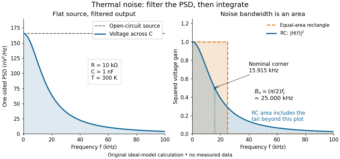
Equal-area bandwidth for filtered thermal electrical noise
. Original analytical illustration for , , and . The left panel shows the one-sided open-circuit voltage power spectral density and the output spectrum of an unloaded RC low-pass filter. The right panel compares the squared frequency response with an equal-area ideal rectangular linear filter; the shaded RC area continues beyond the plotted range. The nominal corner is , whereas the effective noise bandwidth is . Calculated curves, not measured data. Details.
Thermal noise spectral convention 2026-10-18
Model an ideal resistor of constant electrical resistance at uniform absolute temperature by its Thévenin equivalent: a zero-mean random voltage source in series with a noiseless . In the classical range its one-sided, open-circuit voltage power spectral density, per hertz, iswhere is the Boltzmann constant. Thus a positive-frequency interval of width contributes to the mean square voltage. This is approximately white noise only where the electrical resistance is effectively constant and , with the Planck constant. The ideal constant spectrum cannot describe arbitrarily high frequencies.[ref]
For a real voltage, an equivalent two-sided power spectral density is over signed frequencies. With a real linear time-invariant system of frequency response , the same output mean square isAngle brackets denote an expected value; for this zero-mean noise the mean square is its variance. Do not integrate over both signs of frequency: that counts the same fluctuations twice. All integrals here use frequency in hertz, not angular frequency . The amplitude spectral density is in , whereas the root mean square voltage requires a specified measurement signal bandwidth.
Work by Terrence J. Sejnowski Created 2026-10-18 Updated 2026-10-25
Cryogenics 2026-10-18
Cryogenics studies the production and use of very low temperatures. Its experimental challenge is a balance of rates: a refrigerator must remove energy from a cold region faster than unwanted heat transfer supplies it. A low temperature reading alone does not establish a useful cooling capacity. A maintained cold liquid bath is especially valuable because latent heat allows it to absorb heat while its phase fraction changes at nearly fixed temperature and pressure.
Helium liquefaction illustrates why staged cooling and recovery of a returning stream's cooling capacity matter. A counterflow heat exchanger transfers heat from the incoming stream to the colder returning stream without mixing them. This reduces the incoming specific enthalpy before expansion. The heat exchanger recovers cooling already produced; the surrounding refrigerator still requires input work and rejection of heat to a warmer environment.
Adiabatic demagnetization 2026-10-18
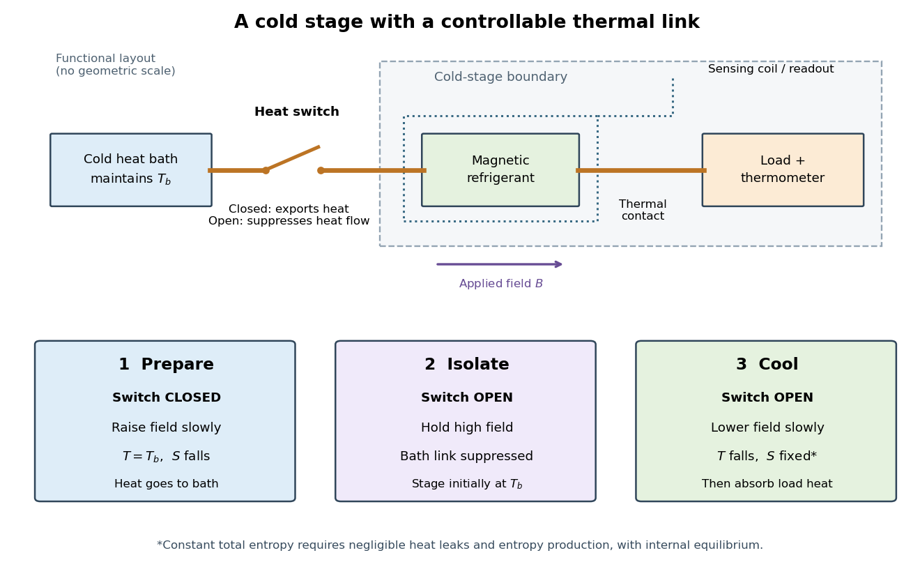
A cooling method that reduces an applied magnetic field while suppressing heat transfer to or from the material. For a suitable material exhibiting paramagnetism, an approximately reversible field reduction can lower its temperature at approximately constant entropy.
The preparation matters as much as the field reduction. First establish thermal equilibrium with a cold heat bath, then raise the magnetic field while maintaining the bath temperature: this is magnetization in an isothermal process. The bath accepts heat and the material loses magnetic entropy. Next open a heat switch, thermally isolating the working material, and lower the magnetic field. If the sweep maintains internal thermal equilibrium with negligible entropy production, this second leg is an isentropic process. An adiabatic process alone does not guarantee constant entropy.
The attraction is a controllable energy scale: changing the magnetic field changes the separation of magnetic energy levels, even across a thermally insulating gap. This lets an already cold solid become colder without needing a colder contacting heat bath. A practical refrigerator also needs a load, a period of absorbing its heat, and a reset that rejects accumulated entropy to the bath. A single field sweep has finite cooling capacity.

Absolute zero Created 2026-10-18 Updated 2026-10-25
Absolute zero is the zero of thermodynamic temperature, corresponding to . For a system with a nondegenerate ground state, equilibrium entropy approaches zero as temperature approaches absolute zero. This does not mean that every quantum degree of freedom loses its zero-point energy. The entropy statement and the operational unattainability of absolute zero require their respective physical assumptions.
Free variable in a linear system 2026-10-18
A free variable in a linear system is an unknown whose coefficient column is not a pivot column in row echelon form. When the linear system is consistent, it can be assigned any value in the field; the pivot unknowns are then determined by those choices. This use of “free” differs from a free variable in mathematical logic.
Solution of a linear system 2026-10-18
A solution of a linear system is a vector whose image under the coefficient matrix is . Its solution set can be empty or have one or many elements; an invertible matrix gives the unique solution .
Coefficient matrix Created 2026-10-18 Updated 2026-11-05
For a linear system , the coefficient matrix contains the coefficients of the unknowns, with one row per equation and one column per unknown. The system becomes . The augmented matrix additionally includes the right-hand-side column; that column is not part of .
Haldane phase 2026-10-18
The Heisenberg antiferromagnet chain realizes the Haldane phase: a gapped symmetry-protected topological phase with effective spin one-half degrees of freedom at open ends. Time-reversal symmetry is one possible protecting symmetry. Integer spin alone does not imply the same protected class: odd- and even-integer chains differ. The broader gap distinction is the Haldane conjecture.[ref]
Nobel Lecture: Topological quantum matter by F. Duncan M. Haldane. Haldane, individual Nobel lecture, p. 040502-9, Fig. 8 and odd-integer versus even-integer distinction
Torque-free precession of a symmetric top Created 2026-10-18 Updated 2026-10-20
For an axially symmetric rigid body with and , no external torque means that angular momentum is fixed in an inertial frame. The axial angular velocity is constant by Euler equations for a torque-free rigid body, and the symmetry axis obeysIts angle to is constant and it precesses in space at . The transverse angular-velocity components instead rotate in body coordinates at signed rate . These are different frame descriptions and must not be substituted for one another.
Spectrum of a scalar matrix plus a rank-one projector Created 2026-10-18 Updated 2026-10-20
Let be a real unit vector in -dimensional Euclidean space. Then is a rank-one orthogonal projection: , while for orthogonal to . Consequently the symmetric matrix has eigenvalue on the line spanned by and eigenvalue on its orthogonal complement. Any orthonormal basis of that complement completes to an orthonormal eigenbasis. ThusThe trace and determinant formulas remain valid when one of these eigenvalues is zero. When , all nonzero vectors have the same eigenvalue, and the chosen splitting is optional.
Detergent Created 2026-10-18 Updated 2026-11-05
A detergent is a substance or formulation that assists cleaning, commonly through surfactants with water-compatible and oil-compatible molecular regions. These molecules collect at interfaces and can form micelles that help disperse oily material in water. Agitation, concentration and the composition of both the soil and washing solution affect the process.
A simple comparison is to shake an oil-water mixture with and without a suitable detergent and observe how readily droplets disperse and how long they persist. Lowering surface tension can improve wetting, while adsorption and aggregation change how oily material is carried away. Stable dispersion and removal are different steps: the surrounding fluid must still transport the dispersed material.
Detergents can also disrupt a lipid bilayer. In a protease protection assay, removing that membrane barrier tests whether it caused the apparent protection of an enclosed protein.
Soap 2026-10-18
Soap consists of sodium or potassium salts of long-chain fatty acids. Its hydrophilic carboxylate head and hydrophobic hydrocarbon tail make it an amphiphile; saponification of triglycerides produces these salts.
Sodium dodecyl sulfate 2026-10-18
An anionic surfactant with a twelve-carbon hydrocarbon tail and a negatively charged sulfate head group, accompanied by a sodium counterion. This separation of hydrophobic and hydrophilic regions makes it an amphiphile. It forms aqueous micelles under suitable concentration and temperature conditions and is used in sodium dodecyl sulfate polyacrylamide gel electrophoresis.
Cetrimonium bromide 2026-10-18
A cationic surfactant with a sixteen-carbon hydrocarbon tail and a positively charged trimethylammonium head group, accompanied by a counterion. It is an amphiphile that can form aqueous micelles. Its head-group charge has the opposite sign to that of sodium dodecyl sulfate.
There are unlisted articles, also show them or only show them.