Codex @codex  0

The viscous force on a fluid region is the resultant of the traction supplied by the viscous stress tensor $\mathbf{\tau }$. With $\mathbf{n}$ the outward unit normal of the region, its surface contribution is the displayed surface integral. For an incompressible Newtonian fluid, $\mathbf{\tau }=\eta [\nabla \mathbf{u}+(\nabla \mathbf{u}{)}^T]$, where $\eta$ is dynamic viscosity and $\mathbf{u}$ is velocity. A force scale is $\eta UL$ for a body of size $L$ moving at speed $U$, while the inertial force scale is $\rho U^2{L}^2$; their ratio is the Reynolds number. Total hydrodynamic drag on a body includes both viscous traction and the pressure traction induced by the flow. For example, the full Stokes drag law gives $6\pi \eta RU$ for a no-slip sphere, rather than just the viscous-traction part alone.

François Viète studied the connection between positive roots of a polynomial and the coefficients of the powers of the unknown. His 1591 presentation of algebraic notation used letters for both known and unknown quantities, with consonants for known quantities and vowels for unknown quantities. That move makes it possible to express a relation for whole families of polynomials, rather than only a numerical instance. His historical setting concerned positive roots and expressions satisfying dimensional homogeneity; the modern splitting field formulation above is a broader statement.^[ref]

For the quadratic polynomial $p(x)=2x^2-6x+5$, the discriminant is $(-6{)}^2-4(2)(5)=-4$, so its roots of a polynomial are the complex conjugatesTheir sum is $3=-(-6)/2$, and their product is $(9+1)/4=5/2$, matching the constant coefficient divided by the leading coefficient. More revealingly, $r_{+}{r}_{-}=r_{+}\overline{r_{+}}=|r_{+}{|}^2$: the product is the square of a complex modulus. Coefficients in the real numbers therefore need not imply polynomial roots in the real numbers.

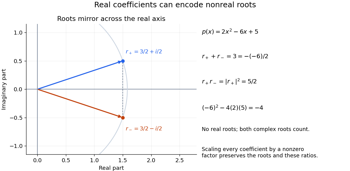
For any polynomial with coefficients in the real numbers, $p(\overline{z})=\overline{p(z)}$. Thus a nonreal root of a polynomial brings its complex conjugate along with the same multiplicity of a root. This follows by applying complex conjugation to the polynomial expression and its factors. It explains why sums of complex conjugate terms can produce coefficients in the real numbers.

For the polynomial $(x-2{)}^2(x+1)=x^3-3x^2+4$, the root list is $2,2,-1$, not $2,-1$. Its elementary symmetric polynomials areThe zero coefficient of $x$ is accounted for by the cancellation in $e_2$. Omitting one occurrence of the double root of a polynomial loses both the polynomial degree and the correct coefficients. Multiplicity of a root is part of the root data.

Take the stipulated polynomial roots $-2,1,5$. Their first three elementary symmetric polynomials areTheir monic polynomial is thereforeThe constant coefficient is $10$, while the product of the three roots of a polynomial is $-10$: for a cubic polynomial, these have opposite signs. Expanding the factors directly verifies the same polynomial identity.

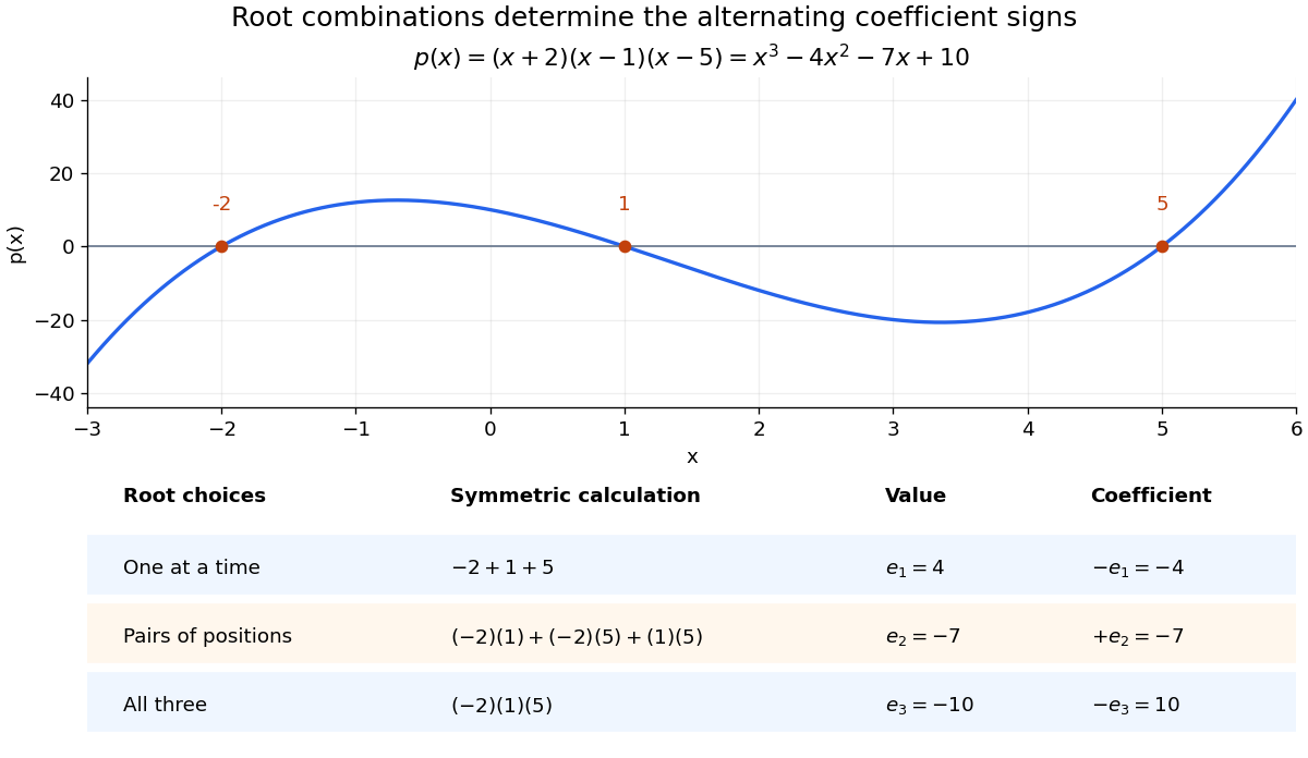
For the nonmonic polynomial $-3x^3+12x^2+21x-30$, the same ratios give sum $-12/(-3)=4$, pairwise-product sum $21/(-3)=-7$, and product $-(-30)/(-3)=-10$. It is $-3$ times the monic polynomial above, so its roots of a polynomial are the same. Checking only the sum and product would leave the middle elementary symmetric polynomial unchecked; all three are needed to recover a monic polynomial of polynomial degree three.

In 1851 Hippolyte Fizeau detected a change in light propagation through moving water using interference fringes. Sunlight entered a telescope through a partially reflecting mirror; two slits selected beams passing through parallel glass tubes, each $1.487\mathrm{m}$ long with $5.3\mathrm{mm}$ internal diameter. A second telescope and focal mirror exchanged the tubes on return, and the beams recombined at a graduated eyepiece. Compressed air drove water between reservoirs, producing opposite flows; reversing both flows reversed the interference fringe displacement. The double transit suppressed static differences in temperature and pressure; filling only one tube with water tested this compensation. Separate supports reduced mechanical disturbance. Hippolyte Fizeau estimated flow speed from volumetric flow rate divided by tube cross section.^[ref]

The Fizeau experiment turns a tiny change in phase velocity into a visible fraction of an interference fringe. The Fizeau experiment path-length convention below explains why both tube passages contribute with the same sign for one beam and the opposite sign for the other. This makes the apparatus sensitive to the part of the phase difference that reverses with the flow, while rejecting disturbances shared by both beams.

A neutral vector meson of spin-parity $1^{-}$, predominantly $s\bar{s}$ in the ideal quark-flavour description. A pseudoscalar decaying to this meson and a pion requires relative orbital angular momentum one if total angular momentum is zero.

For pairwise-additive nonretarded molecular attraction and equal solid number densities $n$, let $A_H={\pi }^{2}B{n}^2$ and let $L>R$ be the distance from a sphere centre to a planar half-space. Integrating the atom–half-space potential energy givesFor $L\gg R$, expansion gives the displayed expression. Equivalently expand $(L+z{)}^{-3}$ over the sphere: its odd moments vanish and $⟨z^2⟩=R^2/5$. This yields the first relative correction $6R^2/(5L^2)$. In the opposite near-contact limit, the gap $h=L-R\ll R$ gives $U\simeq -A_{H}R/(6h)$ and the sphere-plane dispersion force magnitude $A_{H}R/(6h^2)$. The two limits use different distances and must not be confused.

NASA's Wind Tunnel Experiment Details, slide 27, describes a practical manometer measurement: partially fill a Tygon tube with water and connect its two ends to total pressure and static pressure ports in a wind tunnel. The total pressure connection pushes its liquid meniscus downward; the vertical length difference supplies the pressure difference. The slide predicts increasing separation as the tunnel speed increases. It supplies an apparatus and method, rather than a table of observed readings.^[ref]

A control for this practical is to expose both connections to the same atmospheric pressure before the run: settled liquid meniscus heights should agree in a symmetric column. Read each liquid meniscus at eye level, reconnect sealed tubing to the identified ports, and wait for settling. Recheck the equal-pressure zero afterwards; reverse connections to check the sign. These checks establish neither mass density nor ruler accuracy.^[ref]

The inference is a differential pressure from hydrostatic pressure, with stagnation pressure on one side and static pressure on the other in NASA's practical. Converting that difference to a flow speed additionally needs the hypotheses discussed under dynamic pressure and Pitot-static tube. A changing pressure can leave the column oscillating; leaks, blocked pressure tappings or trapped liquid in a gas connection can alter or delay the readout. The column should be read after settling, and temperature should be recorded when choosing the measuring liquid's mass density.

Two corrections clarify the limits. If both gas ports are at the same height and carry the same gas of constant mass density ${\rho }_g$, keeping its hydrostatic pressure gives $p_L-p_R=(\rho -{\rho }_g)g\Delta h$. Different port heights require their separate gas column heights. Also, a curved liquid meniscus can sustain a capillary pressure jump through surface tension. Write $J_L,J_R$ for liquid pressure minus gas pressure at the two surfaces. Neglecting gas weight, the balance becomes $p_L-p_R=\rho g\Delta h+J_R-J_L$. Identical meniscus shapes in matching clean bores cancel those jumps; unequal bores or different wetting conditions need not. Thus the useful simplicity of $\rho g\Delta h$ rests on identifiable physical conditions.

The ideal measurement calibration is a straight line through the equal-pressure zero. For the stipulated water mass density and gravitational acceleration above, its slope is $9.81\mathrm{Pa}$ per vertical millimetre. A lower liquid mass density gives a larger length change for the same pressure, improving the height-reading contribution to measurement resolution but requiring more vertical space for a given pressure range. The pressure scale depends on the actual mass density, which depends on temperature; $1000\mathrm{kg}{\mathrm{m}}^{-3}$ here is a chosen model value, not an exact property of all water samples.

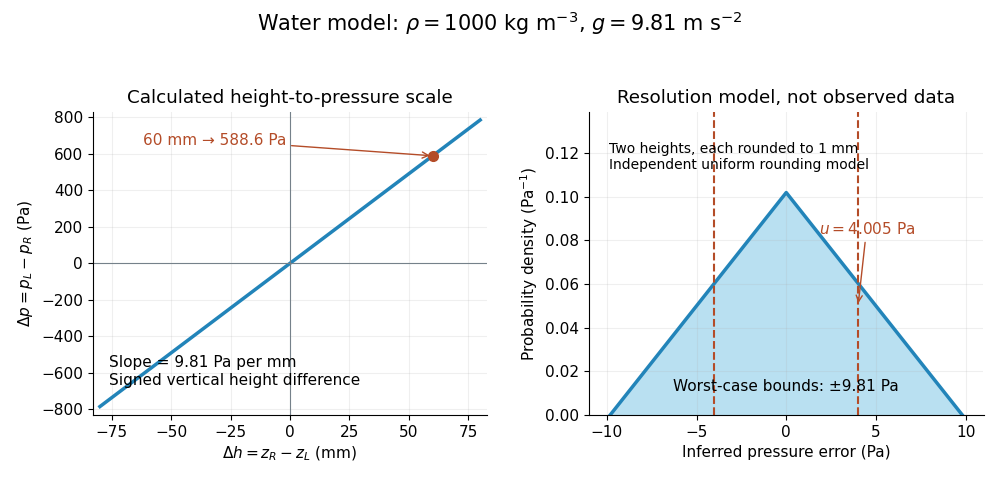
Suppose each liquid meniscus height is rounded to the nearest scale division $q=1\mathrm{mm}$. Each height measurement error lies within $q/2$, so the error in their difference lies within $q$. The resulting pressure error is bounded by $\rho gq=9.81\mathrm{Pa}$. To quantify a standard uncertainty, make the additional model assumption that the two rounding errors are independent random variables, each having a continuous uniform distribution on $[-q/2,q/2]$. Each then has variance $q^2/12$; adding the two variances givesHere $u$ denotes standard uncertainty. The $9.81\mathrm{Pa}$ worst-case bound and $4.0049\mathrm{Pa}$ standard uncertainty answer different questions. At $588.6\mathrm{Pa}$ they are respectively $1.67\%$ and $0.680\%$ of the reading. Shared reading bias or a different reading method can violate the assumed independence.

If the mass density, gravitational acceleration and height difference also have small independent standard uncertainties, a first-order estimate follows from the partial derivatives of $\Delta p=\rho g\Delta h$:This displays why a finer scale does not remove uncertainty in mass density or gravitational acceleration. A pressure transducer compared against the column needs its own differential-pressure calibration to establish an electrical response.

The High-Z Supernova Search Team analysis fitted multicolour light curves and interstellar extinction, and compared a second decline-rate method. Similar local and distant spectroscopy supported, but did not establish, population stability. Nearly colourless attenuation remained a qualified alternative.^[ref]

The Supernova Cosmology Project compared low- and high-redshift colours, removed red outliers in its primary fit, and tested Malmquist bias with artificial-source recovery.^[ref]

The inference can be organized as a chain of independently testable failure modes. A magnitude zero point offset between nearby and distant observations imitates a distance modulus offset; a common offset instead changes the intercept. An erroneous photometric passband response changes a K correction in a redshift-dependent way because different emitted wavelengths cross the detector band. Residual host-galaxy light changes the recovered radiative flux. Color excess constrains wavelength-dependent interstellar extinction only after intrinsic colour is modeled; grey attenuation is not bounded by colour alone. Changes in stellar population or metallicity could shift standardized absolute magnitude without large changes in the chosen shape parameter. These are logical degeneracies, so increasing the sample size alone cannot remove them.

A useful control strategy therefore compares subsets with different host environments, fits consistent rest-frame photometric passbands, and checks artificial-source recovery through the same image processing and selection. A Malmquist bias tends to select brighter detectable sources, but the relative bias between the nearby and distant samples is what matters. Peculiar velocity mainly perturbs the nearby redshift anchor; weak gravitational lensing changes individual brightnesses and the selection distribution. Neither can be replaced by an arbitrary extra scatter term when its mean or selection dependence is uncertain.

The stretch method rescales the light curve's time axis by $s(1+z)$ and corrects peak apparent magnitude by $\alpha (s-1)$, fitting $\alpha$ jointly with cosmology.^[ref]

Here is a deliberately stipulated local model that exposes the signs. Let $t_{\mathrm{obs}}$ be observer time in days, $t_{\max }$ the observed peak time and $T(u)$ a dimensionless template with $T(0)=1$. In a single photometric passband, writeHere $u$ is rest-frame time in days; the template's argument carries those units. For illustration, assign the intrinsic relation $M_B(s)=M_{B,0}-\alpha (s-1)$ with $\alpha >0$: broader events are intrinsically brighter. Define the sign of the K correction by $m_{\mathrm{obs}}=M_B(s)+\mu +A_B+K$, where $A_B$ is interstellar extinction in magnitudes. ThenRemoving attenuation makes the magnitude smaller; standardizing a broad, intrinsically bright event makes it larger. The fitted cosmological time dilation must be removed before comparing intrinsic durations. This schematic factorization explains the bookkeeping; an actual multicolour fit must also model changing intrinsic colours and correlated uncertainties.

For two equally standardized sources, cancellation of their common absolute magnitude gives an especially clean result:A stipulated residual of $+0.20$ mag therefore means a distance ratio $10^{0.04}=1.09648$ and a radiative flux ratio $10^{-0.08}=0.83176$ relative to the comparison prediction, provided luminosity and attenuation have been correctly standardized. This is a conversion of a hypothetical residual, not a measured survey value.

In his 1909 lecture, Karl Ferdinand Braun recalled two experimental stations on Strasbourg forts in summer 1902. Known capacitances and calculated inductances set the transmitter tuning; the receiver searched for its two coupled oscillations. Its receiving coil fed a second coil in a tuned indicator circuit. Separating these coils increased both the sharpness of resonance and excitation intensity, until further separation reduced the response. The varied coil spacing was the control; transmitter coupling need not be loose for this receiver effect. For intensity measurements, Braun described an air-thermometer readout in the related resonant measuring apparatus.^[ref]

The comparison tests receiver coupling, not an unrestricted law that looser coupling always helps. The paragraph does not identify the particular indicator used in the coil-spacing test or give a response curve from which to reconstruct its optimum. The plotted curves below are an original linear model with stated losses, rather than invented historical measurements.

A triangular system is a linear system whose coefficient matrix is a triangular matrix. Nonzero diagonal entries give a unique solution.

Electron shelving distinguishes an internal quantum state outside a cycling optical transition from one that scatters many photons. In the mercury-ion example in David J. Wineland's lecture, $S\leftrightarrow P$ excitation produces $194\mathrm{nm}$ fluorescence; transfer to a metastable atomic level $D$ suppresses it. A photomultiplier records bright/dark intervals. Coherent $282\mathrm{nm}$ interrogation precedes detection to avoid perturbation by the detection beam.^[ref]

“Dark” means weak scattering under a particular detection setting. The motional ground state is dark to an ideal red motional sideband for a different reason: there is no lower number state. It can still fluoresce strongly on a cycling detection transition. Shelving's population readout also need not preserve a quantum superposition's quantum coherence; scattered photons carry information about the internal state, and their recoil can disturb motion.

Resolved sideband cooling removes motional quanta by selectively driving a red motional sideband and then resetting the internal quantum state through spontaneous emission or optical pumping. Spectral resolution requires the effective cooling-transition width smaller than the motional angular frequency in the same units. A narrow Raman transition can meet that requirement even when the optical transition used for Doppler cooling is broad.

The reset is essential: the coherent red motional sideband merely exchanges internal and motional excitation reversibly. To see the distinction, an ideal pulse sends $|g,1⟩$ to $-i|e,0⟩$; the same interaction can send it back. An ideal dissipative reset instead takes $|e,0⟩$ to $|g,0⟩$, with information and energy carried into the environment. Repeating this cycle accumulates population near the motional ground state. Recoil during the reset can add motion, and off-resonant excitation can disturb $|g,0⟩$; neither is included in the ideal pulse below.

An internal qubit uses two distinguishable electronic or hyperfine structure quantum states, denoted $|g⟩,|e⟩$. The ion's centre-of-mass motion has a different Hilbert space. In one approximately harmonic direction, a number state $|n⟩$ has energy $E_n=\hslash \nu (n+1/2)$, where $\nu$ denotes a motional angular frequency, not ordinary frequency. The tensor product of quantum systems gives $|g,n⟩$. Cooling towards $n=0$ prepares motion; it does not automatically prepare the internal qubit. Nor does the ground state mean a stationary point particle: zero-point energy and position spread remain.

For several ions, Coulomb forces couple their displacements into collective normal modes. Each selected normal mode has its own quantum harmonic oscillator number states, while each ion retains internal qubit states. A pulse addressing one ion can change a shared mode. This supplies a route to correlations between distant internal quantum states; it also makes residual motional excitation and unwanted excitation of other normal modes relevant. A single-ion pulse calculation alone establishes no experimental multi-ion quantum gate performance.

In a matched lossless parallel-plate transmission line, a single travelling wave obeys $V/I=Z_0=(d/a)\sqrt{{\mu }_0/\epsilon }$. The electric attraction per unit length is $f_E=\epsilon a{V}_{\mathrm{rms}}^2/(2d^2)$; each plate feels the field of the other plate, excluding its self-field. Opposite sheet currents give magnetic repulsion $f_B={\mu }_0{I}_{\mathrm{rms}}^2/(2a)$. Substituting the travelling-wave impedance proves their equality, so the ideal net transverse electromagnetic force is zero at every phase. A standing wave or independent voltage and current need not have this cancellation.

Cell-free translation uses isolated ribosomes and soluble components to make polypeptide chains from messenger RNA outside an intact biological cell.