
Defocus aberration 2026-10-14
Defocus is the mismatch between the receiving plane and the intended optical focus. Changing the plane changes the point spread function even when the optical lens is otherwise ideal.
Airy disk Created 2026-10-14 Updated 2026-10-14
The Airy disk is the central bright region, up to the first dark ring, in the scalar diffraction pattern of a uniformly illuminated, unobscured circular aperture. The whole pattern includes the weaker surrounding rings; its radius is distinct from its full width at half maximum.
For a circular optical pupil of diameter under normal, uniform monochromatic plane wave illumination, Fraunhofer diffraction givesHere is the on-axis light intensity, is the angle from the optical axis, is the wavelength in the propagation medium, and is the order-one Bessel function of the first kind. The paraxial approximation replaces by , measured in radians. The first positive zero givesThis is the angular radius of the Airy disk; the angular diameter is twice as large. The Airy disk derivation explains the origin of the Bessel function of the first kind and of the numerical coefficient.[ref]
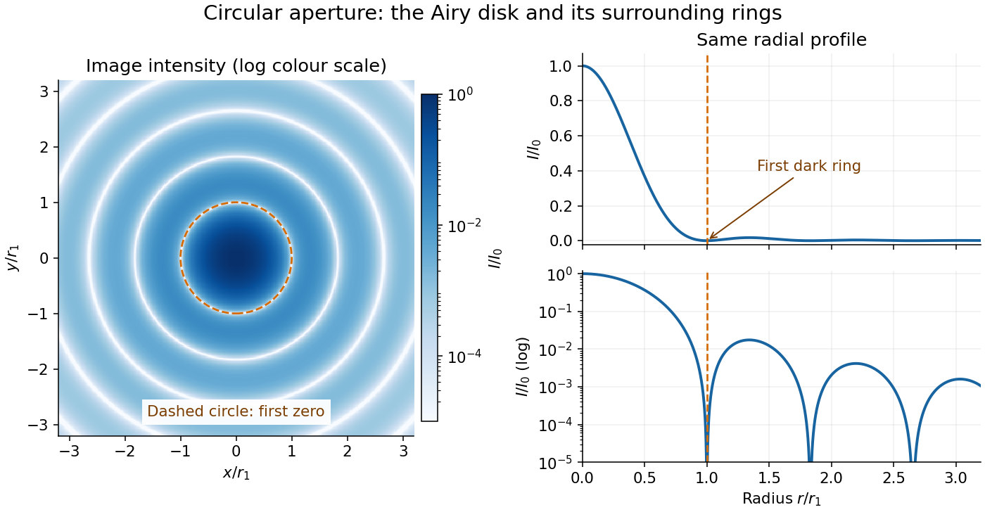

The image and both radial curves show the same calculated light intensity, divided by its peak. The image's logarithmic scale makes the weak rings visible; its colour is a display choice. The linear curve shows how small the ring peaks are compared with the centre. A dark ring marks a zero of wave amplitude, produced by cancellation across the optical pupil; it is not the edge of all transmitted light. The first Airy disk contains about of the total radiant flux, as calculated in Airy disk normalization and encircled energy.
For an original design example, take an ideal optical lens in air with focal length , circular optical pupil diameter and wavelength . In the focal plane, the radial coordinate givesThe first-zero diameter is . Solving gives , so the diameter measured by full width at half maximum is onlyThus a quoted “spot diameter” is incomplete without its definition. Doubling halves both widths at fixed wavelength and focal length; increasing magnification alone changes the image scale without improving object-space discrimination.
The Airy disk supplies a calculable reference for a point spread function, allowing diffraction to be distinguished from defocus and optical aberrations. Its beauty is that one circular boundary determines an entire sequence of bright and dark rings through a Fourier transform. The ideal formula assumes an unobscured pupil, uniform illumination, ideal optical focus, a single wavelength, and a scalar description with small output angles. A blocked centre, nonuniform pupil transmission or a significant pupil wave phase error changes the response. High numerical aperture may require polarization of an electromagnetic wave and a vector field description. The circular-aperture diffraction laboratory experiment tests the far-field pattern directly; the Rayleigh criterion uses its first zero to define a two-source convention.
Coherent imaging 2026-10-14
In coherent imaging, complex wave amplitudes add with their relative wave phases preserved. The measured light intensity includes wave interference between the contributions.
Incoherent imaging 2026-10-14
In incoherent imaging, contributions from distinct object points add as light intensities because their mutual spatial optical coherence is negligible. A single convolution additionally requires translation invariance of the point spread function.
Optical point source 2026-10-14
An optical point source has spatial extent negligible relative to the imaging scale being tested. The Dirac delta function is its idealization; a finite bead or unresolved star only approximates it.
Point spread function normalization Created 2026-10-14 Updated 2026-10-14
Point spread function normalization specifies how the response is scaled. Unit-integral scaling separates image shape from total radiant flux; unit-peak scaling compares shapes but does not make their total radiant fluxes equal.
Hydrodynamic attraction of a plane wall to a point source Created 2026-10-14 Updated 2026-11-05
An incompressible point source of volume flux at height above an impermeable plane has velocity potential , with an equal image source below the plane. On the wall, . The Bernoulli equation gives . Integrating the pressure deficit over the plane gives the displayed attraction force relative to ambient pressure. If source strength instead denotes the coefficient of radial inverse-square velocity, the force is .
Three-dimensional point source Created 2026-10-14 Updated 2026-11-05
A point injection of volume at rate produces the displayed radial potential flow in three dimensions. Its velocity potential is , and every enclosing sphere has outward volume flux . The divergence vanishes away from the source and is times the three-dimensional Dirac delta distribution at it. The field is also a Stokes flow with constant pressure away from its singularity.
Source dipole Created 2026-10-14 Updated 2026-11-05
A source dipole is the limit of an equal source and sink brought together with their source-strength times separation vector fixed at . Differentiating the three-dimensional point source field gives . It has velocity potential , zero total volume flux, and far-field decay. Unlike a stresslet, it is an irrotational potential singularity rather than a force-dipole flow.
Simple locally finite point measure 2026-10-14
A point measure is a countable sum of Dirac measures. It is simple if all its atoms have mass one, and locally finite if every bounded set has finite mass. Simplicity lets fine enough cells count individual points, whereas occupation indicators would lose multiplicities in a nonsimple measure.
Void probability functional Created 2026-10-14 Updated 2026-11-05
The void probability functional assigns to a measurable set the probability that it contains no atom of a random point measure. For a Poisson random measure of intensity , it is . The exponential void probabilities characterize a Poisson random measure result uses simplicity; doubling every atom of a Poisson measure preserves void probabilities but changes count distributions.
Intensity measure of a point process 2026-10-14
The intensity measure of a point process is its expected counting measure:It may take the value .[ref]
Lectures on the Poisson Process by Günter Last and others. Section 2.2, Definition 2.5, printed p. 12: intensity as the expected counting measure
Countable additivity follows by applying the monotone convergence theorem to the counts of finite unions of pairwise disjoint observation windows. If is locally finite and absolutely continuous with respect to Lebesgue measure, its Radon-Nikodym derivative is the intensity function of a point process :This is an expected number per unit volume, not a probability density function for a randomly selected point. For example, a single deterministic point has , a Dirac measure, and no Lebesgue measure density. The density representation requires its own assumption.[ref]Spatial Point Processes and their Applications. Section 2.1, Definitions 2.1-2.2, printed pp. 26-27: expected counts and intensity functions
For a bounded Borel set , , but local finiteness alone does not ensure that this expected value is finite. Conversely, implies almost surely, even when is unbounded. A constant finite intensity function of a point process on all of has infinite total intensity measure, although every bounded window has finite expected value.
Neyman-Scott process Created 2026-10-14 Updated 2026-11-05
A Neyman-Scott process places independent offspring clusters around points of a Poisson parent process, with an independently drawn offspring count and displacements. Poisson offspring counts make the offspring process conditionally Poisson given the parents, and therefore give a Cox process. Arbitrary offspring counts need not have that property.
Stationary point process 2026-10-14
A point process on is stationary if every translation preserves its probability law. If its mean count in a unit cube is finite, its intensity measure is for some , where denotes Lebesgue measure. This follows because stationarity makes the mean measure invariant under translations. A constant intensity function of a point process describes only these mean counts, and by itself asserts neither stationarity of the entire law nor independence.[ref]
Lectures on the Poisson Process by Günter Last and others. Section 8.1, Proposition 8.2, printed pp. 69-70: stationarity and constant intensity under a finite unit-cube mean
Window count of a point process 2026-10-14
For a bounded Borel set , the window count of a locally finite point process is a finite nonnegative integer random variable. It counts multiplicities, and the convention for window boundaries matters. On the time half-line, is a counting process and . For pairwise disjoint observation windows , the measure identityis valid for every realization. Additivity of counts supplies no independence assumption.
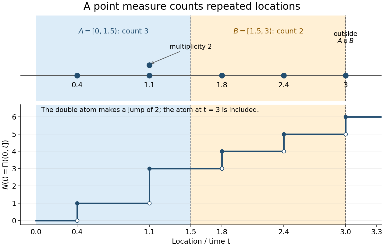
Window counts include multiplicity and depend on boundary conventions
. One locally finite point measure is . The half-open windows and have counts three and two; . The atom at three lies outside both windows. Two stacked dots denote the double atom at , and the step plot records , which includes the atom at three. Details.
Simple point process 2026-10-14
A point process is simple when, on a single almost sure event, every location has multiplicity at most one. Its realizations are simple locally finite point measures. For instance, is locally finite but not simple: it has four points counted with multiplicity at three distinct locations. Simplicity is a statement about each entire realization. Checking separately for every fixed is insufficient: with having the uniform distribution on passes every such fixed-location check, yet always has a double point.[ref]
Lectures on the Poisson Process by Günter Last and others. Section 6.2, Definitions 6.6 and 6.8, printed p. 49: simple measures and simple point processes
Crystallographic restriction theorem Created 2026-10-14 Updated 2026-10-20
Poincaré horizon 2026-10-14
The boundary of a chosen Poincare coordinates on anti-de Sitter spacetime patch inside the full spacetime is a null coordinate horizon. It is not the timelike conformal boundary, and not a curvature singularity. Timelike geodesics can cross it in finite proper time while the patch time diverges. In a signed-diameter conformal strip, the patch containing satisfies .
For unit-radius metric , translations conserve . Timelike normalization gives and . Setting yields , hence the displayed proper-time solution where the cosine is positive. Its two patch-horizon crossings are separated by proper time , although the globally extended geodesic is complete.
Conjunction (astronomy) 2026-10-14
An astronomical conjunction occurs when two orbiting bodies have the same apparent longitude as viewed from their primary or from an observer.
There are unlisted articles, also show them or only show them.