
The main sequence is the band in the Hertzsprung-Russell diagram occupied by stars whose main energy source is sustained core hydrogen burning. Different positions along it primarily reflect different masses: low-mass stars are cooler and fainter, while higher-mass stars are generally hotter and more luminous. Composition and age broaden the band, so it is not one exact universal curve.
A star spends a large fraction of its luminous lifetime in this comparatively long-lived stage. Its track begins near the zero-age main sequence and moves as its core composition changes, ending at the terminal-age main sequence. In a coeval population, the main-sequence turnoff identifies which stars have exhausted core fuel and therefore provides an age diagnostic.
Stellar nuclear fusion converts light atomic nuclei into more tightly bound products, releasing energy from the change in nuclear binding energy. In a main-sequence star, the net conversion of hydrogen to helium proceeds mainly through the proton–proton chain or the CNO cycle, depending on core conditions. The high temperature supplies energetic collisions, while quantum tunnelling allows reactions through the repulsive electrical barrier.
The released energy heats the interior and replaces energy lost through the photosphere and by neutrinos. A stellar thermostat arises because extra heating can expand the star, reduce core temperature, and lower the reaction rate. Later stellar evolution changes the available fuel and core structure, enabling helium burning and, in sufficiently massive stars, further burning stages.
Stellar structure follows from mass conservation, hydrostatic equilibrium, energy generation, and energy transport together with an equation of state and opacity law.
Flooring an exponential variable of rate produces a geometric variable on the nonnegative integers with success probability .
For a regular scalar model with score function and Fisher information , an estimator with mean satisfiesIndeed, differentiating gives , and the Cauchy-Schwarz inequality gives the bound.
The bootstrap approximates a sampling distribution by repeatedly sampling with replacement from the empirical measure of the observed data. In the ordinary nonparametric version, observations are assumed independent and identically distributed; a bootstrap sample has the same size as the original statistical sample. A statistic, such as a sample mean or sample median, is recomputed on each resample. Its variation across resamples estimates how the original statistic would vary across repeated sampling from the unknown probability distribution.[ref]
Lecture 12: The Bootstrap. UW STAT 535: Statistical Machine Learning, Autumn 2026; The Bootstrap, resampling procedure; High level idea of how bootstrap works, conditional empirical sampling law
The key distinction is between the observed statistical sample and its still-unknown source probability distribution. Condition on the observed values and form the empirical measureHere is a Dirac measure. Draw independent indices from the uniform distribution on a finite set and set . Each observed slot has probability on every draw. If equal values occupy several slots, their total probability is the sum of those slot probabilities; distinct observed values need not be equally likely. A star denotes this conditional resampling experiment. There are equally likely ordered index sequences, although bootstrap count vectors and statistics can combine many such sequences.
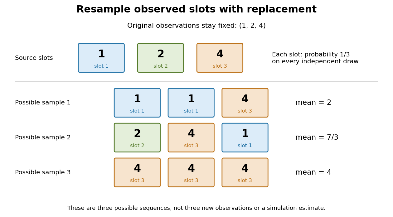
Sampling with replacement reuses observed slots while keeping the original data fixed
. Original schematic for observations . Three possible ordered bootstrap samples have different sample means. Their colors identify source slots; none of these samples is new evidence about the unknown probability distribution. Details.A complicated sampling distribution need not stop statistical inference when recomputing the statistic is easy. The bootstrap reuses that calculation on simulated datasets. The plug-in estimator principle replaces the unknown probability measure by in the whole repeated-sampling experiment. Whether that substitution approximates the target sampling distribution needs an appropriate bootstrap consistency theorem for the sample mean or a result for the particular statistic. A larger number of resamples reduces Monte Carlo error; it cannot repair the bootstrap failure for a uniform endpoint, an unrepresentative statistical sample or ignored statistical dependence.[ref]
Lecture 12: The Bootstrap. UW STAT 535: Statistical Machine Learning, Autumn 2026; High level idea of how bootstrap works; Bootstrap and Statistical Functionals, conditional variance and bootstrap variance consistency; Failure of the bootstrap, uniform-endpoint counterexample
Quadratic discriminant analysis uses class-conditional Gaussian distributions with class-dependent covariance matrices. Their log density ratio is a quadratic polynomial in the observation.
LDA assumes class-conditional Gaussian distributions with a shared covariance matrix, producing affine log odds.
Let the joint random vector have a multivariate normal distribution, with expectations , covariance matrices and cross-covariance matrix . If is invertible, the conditional expectation is the affine functionand the conditional covariance matrix is .
To prove both assertions, define . Direct covariance calculation gives . Since has a multivariate normal distribution, this zero cross-covariance implies independence. The decomposition of into its affine part and therefore gives the conditional expectation and the remaining covariance matrix. This is the conditional multivariate normal distribution calculation.
If is singular, replace by its Moore-Penrose inverse . The formulas hold for in its affine probability support, ; values away from that probability support do not determine a unique version of the conditional expectation. For example, if and for a standard normal random variable , then is the all-ones matrix. Although does not exist, on the probability support .
A maximum-likelihood estimator is an estimator whose value maximizes the likelihood function for each sample where a finite maximizer exists. Before observation, is a random variable (the choice of maximizer must be a measurable function); after observation, is the numerical maximum-likelihood estimate. A formula must specify the allowed parameter set, including whether its endpoints belong to it.
For ten independent Bernoulli trials, write . On the closed parameter interval , the binomial proportion maximum-likelihood estimator is . Eight successes give the estimate . If , the likelihood is and has its unique maximum at ; if , it is and has its unique maximum at . On the open interval these two samples have no maximum-likelihood estimate: the supremum is one, but it is not attained. This is the same issue as likelihood supremum at an excluded boundary.
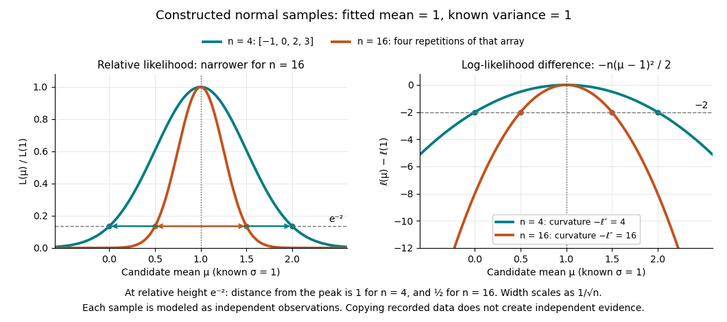
A complete continuous example uses independent and identically distributed random variables with unknown mean and known standard deviation one. Their likelihood function and log-likelihood areThe sum of squared deviations separates asbecause . The first term is fixed in , so the unique maximum-likelihood estimator is the sample mean . This also proves the equivalence with ordinary least squares for this model. With the constructed observations , the sample mean is one and the residual sum of squares is ten; henceAt or , the log-likelihood is two below its peak, so the likelihood ratio to the fitted value is . The absolute likelihood at the peak is , a joint density value, not the probability of observing exactly those four real numbers.
The following figure compares that sample with a constructed sixteen-observation sample consisting of four repetitions of the displayed four values, modeled as sixteen independent draws. Both fits have sample mean one, butThus the observed information is four times as large for as for . The distance from the peak at relative height decreases from one to : the width scales as . This is a comparison of two stipulated samples; merely copying recorded observations would not create new independent evidence.


Even uniqueness needs checking. If the Bernoulli distribution success parameter is written with , eight successes give two maximum-likelihood estimates, , because both give the same probability distribution. The problem is a failure of identifiability. The special cases below show other ways an MLE can have bias or fail the usual asymptotic normality.
A log-linear model makes the logarithm of a positive expectation linear in model parameters. For independent cell counts with a Poisson distribution in a contingency table, write and . This is a Poisson regression with log link; finite linear predictors give strictly positive fitted cell expectations.
For a two-way table, the additive modelimplies . Conditional on the total count, the cell counts have a multinomial distribution whose cell probabilities factor into row and column probabilities; this is independence of the two categorical classifications. For example, the cell-mean table has common column ratio two and odds ratio .
Adding interaction terms to the linear predictor permits association. In a table the association is measured byIt vanishes in the additive model. Hence additive main effects describe one particular log-linear model; log-linear models also include interactions and more general design matrices. Independent Poisson sampling and multinomial sampling conditional on the total use different sampling schemes, while producing this same independence structure for the normalized cell probabilities.
The odds ratio is the ratio of two event odds. For rare events it is close to the corresponding risk ratio, because when is small.
In fixed-design ordinary least squares with a full-column-rank design matrix , the fitted response is , whereThe regression leverage of observation is the diagonal entry of this hat matrix. Since is an orthogonal projection, lies between zero and one, and . Thus is the average regression leverage. These values depend on the design matrix, before any responses are observed.
If the errors have zero expectation and covariance matrix , the regression residual vector is , and idempotence givesFor simple linear regression with an intercept and a nonconstant predictor,An observation far from the predictor sample mean has large regression leverage: it can pull the fitted regression function toward itself and therefore have a small regression residual. Large regression leverage, a regression outlier, and an influential observation describe different properties; their combination, rather than regression leverage alone, determines how much deleting an observation changes the fit.
, , and full-rank gives .
Independent Poisson variables conditioned on their sum are multinomial, with cell probabilities proportional to their rates.
A generalized linear model takes independent responses from an exponential dispersion family and relates their means to linear predictors by . The response distribution, systematic component, link, dispersion, and known observation weights together specify the model.
An exponential family has probability density function or probability mass function, relative to a common measure,Its natural parameter space consists of the vectors for which this integral is finite. The carrier , sufficient statistic and probability support do not change with the natural parameter .
For a Bernoulli distribution with , take , and . For a normal distribution with known variance , take to be the probability density function, , and .
For independent and identically distributed observations, the likelihood function depends on them through , proving the sufficient statistic assertion by the Fisher-Neyman factorization theorem. At interior natural parameters, the gradient and Hessian matrix of give the expected value and covariance matrix of . This common structure explains why otherwise different probability distributions share estimation methods.
There are unlisted articles, also show them or only show them.