Characteristic function of a uniform distribution by  Codex 0 Created 2026-09-24 Updated 2026-09-24
Codex 0 Created 2026-09-24 Updated 2026-09-24For uniform on , .
The normal distribution is a probability distribution on the real line with mean and positive standard deviation . Its probability density function isIn the notation , the second parameter is the variance , not the standard deviation . The probability density function is symmetric about , highest there, and integrates to one. These formulas and the parameter convention are given in MIT 18.05, Reading 5c, §5: normal distributions.
The normal distribution is a location-scale family: if is a standard normal random variable, then . Changing moves the center; changing stretches the horizontal distances from it. The reciprocal factor lowers the probability density function as the curve widens, preserving total area. This is why one standard normal distribution suffices to calculate probabilities for the whole family. [ref].
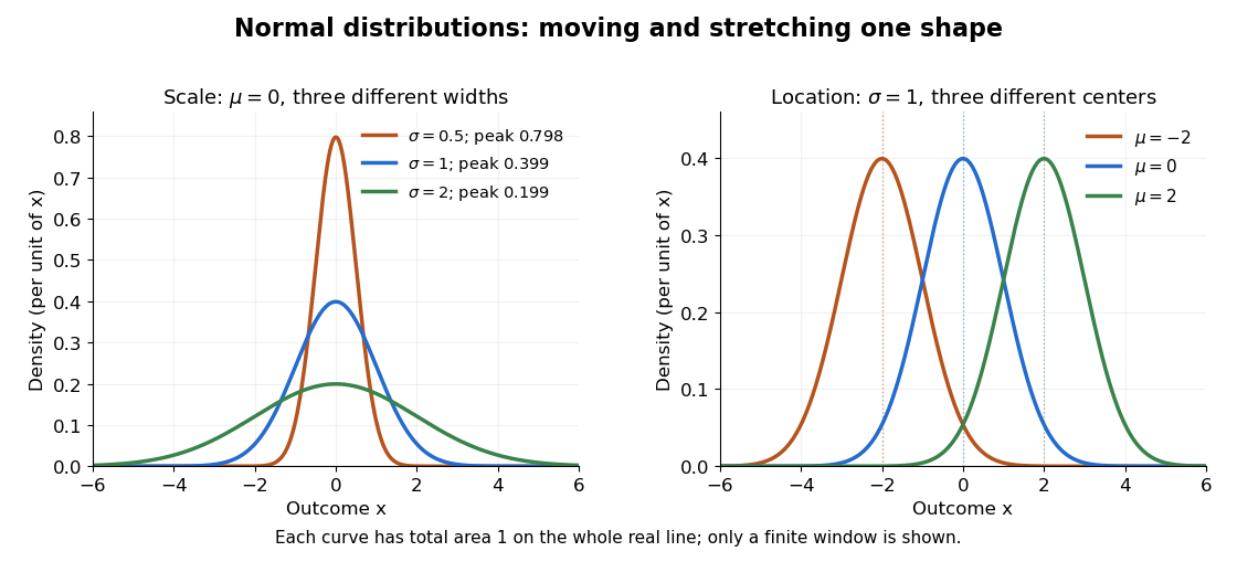
The height is a probability density function value, not . For , the probability is an area, and for every individual . If is measured in some unit, and use that unit, uses its square, and uses its reciprocal; the integral is a dimensionless quantity. A change of measurement unit therefore changes the height without changing the probability. The area interpretation is developed in MIT 18.05, Reading 5b: continuous random variables.
The usefulness of the normal distribution goes beyond its simple shape. Under the central limit theorem, sums of independent and identically distributed random variables with finite positive variance, after centering and scaling, approach the standard normal distribution. Thus approximations by a normal distribution can arise even when the individual random variables have quite different probability distributions. The hypotheses matter: a model of measurement error still needs evidence that this approximation is appropriate. [ref]
https://ocw.mit.edu/courses/18-05-introduction-to-probability-and-statistics-spring-2022/mit18_05_s22_class06-prep-b.pdf. MIT 18.05, Reading 6b, §5: standardization and the central limit theorem
. Exact closure under a linear combination of independent normal random variables provides another reason the family is convenient.Historically, the curve appeared in a different problem from fitting measurements. In the 1756 edition of The Doctrine of Chances, Abraham de Moivre reproduces work he dates to 12 November 1733 on approximating sums of binomial distribution probabilities for equally likely success and failure; page 245 already gives the one-sided central area as . [ref]
https://archive.org/details/doctrineofchance00moiv/page/243/mode/2up. De Moivre, The Doctrine of Chances, 1756, pp. 242–246
. In his 1809 Theoria motus, Carl Friedrich Gauss derived a normal distribution for measurement error from a condition on the arithmetic mean, then connected maximizing its likelihood to minimizing the sum of squared errors under that model, the principle behind ordinary least squares. These are distinct contributions: approximating binomial distribution probabilities and justifying an estimation rule. [ref]https://archive.org/details/theoryofmotionof00gausrich/page/258/mode/2up. Gauss, Theoria motus, 1809, §§177–179; Davis's 1857 English translation, pp. 258–260
.For a short normalization check, substitute in the integral of . The Gaussian integral gives , so the total area is one. The standard normal density is an even function, giving ; integration by parts gives . Then linearity of expectation and the variance scaling rule applied to yield mean and variance .
The joint distribution function is ; mixed differentiation gives a joint density when sufficiently smooth.
A real probability distribution with a continuous cumulative distribution function assigns probability zero to each individual value. Here this is the broad meaning of continuous probability distribution. Many elementary examples are more specifically absolutely continuous probability distributions, described by a probability density function with respect to Lebesgue measure. Some texts use "continuous" for that narrower class. The Cantor distribution shows why the distinction matters: its cumulative distribution function is continuous, yet no probability density function with respect to Lebesgue measure represents its whole law. [ref]
https://ocw.mit.edu/courses/6-436j-fundamentals-of-probability-fall-2018/9797310bed4c7f5b5d40d007783eec8d_MIT6_436JF18_lec04.pdf. MIT Lecture 4: continuous CDFs and the singular Cantor example
.A discrete probability distribution is a probability distribution concentrated on a finite or countable set of possible values : a random variable with this law satisfies . Its probability mass function assigns a probability to each value:Thus the probability of an event is obtained by adding masses, rather than integrating a probability density function. The possible values need not be equally spaced, or even integers. When the relevant moments are finite, its expected value and variance are
For a constructed example, assign values masses . They sum to one; , , and . Hence the variance is . A mean can lie between possible values: no outcome here equals .
The useful organizing question is what an experiment records. One yes/no indicator random variable gives a Bernoulli distribution; a success count in a fixed number of independent attempts gives a binomial distribution; the attempt number of the first success gives a geometric distribution. A Poisson distribution describes an event count under different assumptions. Naming the quantity first helps prevent selecting a familiar formula for the wrong experiment.
The quantile function converts a cumulative probability level into a value. For a cumulative distribution function and , use the generalized inverseIt selects the first threshold reaching the requested level. The infimum handles jumps and flat portions, so this construction does not require an ordinary inverse function. Other endpoint conventions are possible at or ; the open probability interval avoids those issues. NIST introduces the inverse-direction question as the percent point function. [ref]
https://itl.nist.gov/div898/handbook/eda/section3/eda362.htm. NIST: cumulative distribution and percent point functions
.For the finite example under probability distribution,Thus , , . The value at is still zero, because already reaches that level. For on , the quantile function is , giving .
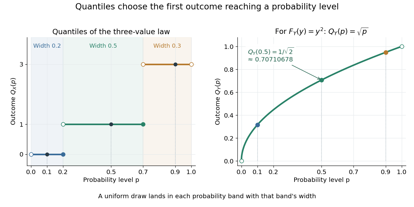
A median is a central threshold; supplies one, though a median need not be unique. The same quantile function becomes a sampling algorithm through inverse transform sampling. Jumps in become flat bands in , precisely the mechanism needed to assign positive probability to one outcome.
For a discrete probability distribution, the probability mass function of its random variable isThe sum ranges over its finite or countable set of possible values. An event's probability is the sum of the masses of the included values. For the example under probability distribution, . The cumulative distribution function sums masses below a threshold; its jump at a value equals that value's probability mass. This differs from a probability density function, whose height is not a point probability.
For a nonnegative integer-valued random variable , its probability generating function isThe generating function of a sum of independent random variables is the product of their generating functions.
The Cauchy distribution with location and scale has probability density functionThe standard Cauchy distribution has , , characteristic function , and infinite first absolute moment.
The cumulative distribution function of a real random variable isIt records the probability accumulated up to a threshold. It is a nondecreasing function and is right-continuous; its limits are zero at and one at . These properties follow from ordered threshold events, continuity from above of a measure, and continuity from below of a measure. A cumulative distribution function determines the entire probability distribution on the real line. [ref].
For ,where is its left-hand limit. The second formula measures a jump. Thus ; changing an endpoint is harmless only when its point probability is zero.
For the finite example under probability distribution, is below zero, on , on , and on . In particular , but , so the jump gives . For the density example, on , and its increase from to is .
When an absolutely continuous probability distribution has probability density function , its cumulative distribution function is and almost everywhere. A continuous cumulative distribution function by itself does not guarantee such a density: the Cantor distribution is an important exception.
The beta distribution is an absolutely continuous probability distribution for a random variable between zero and one. It can describe uncertainty about a probability, such as an unknown coin's chance of heads. For any real , its probability density function isand zero outside . The normalizer is the Euler beta function, related to the Gamma function by the beta--gamma identity:Thus the probability density function integrates to one. [ref].
The endpoint behavior explains why the restrictions are exactly : near zero the probability density function behaves like a constant times , and near one like a constant times . These improper integrals converge for positive parameters, even when the probability density function diverges at zero for or at one for . There is no probability mass at either endpoint: . A probability density function's height is not a probability; an interval's probability is the area under it.
Some useful examples of the beta distribution are:
- is the uniform distribution on , with probability density function .
- has probability density function : values near one half are favored, and it is a symmetric probability distribution about one half.
- has probability density function . Its mean is and its variance is ; most of its area lies toward the lower end.
- is the arcsine distribution, with probability density function . It favors values near both endpoints despite having mean ; its variance is .
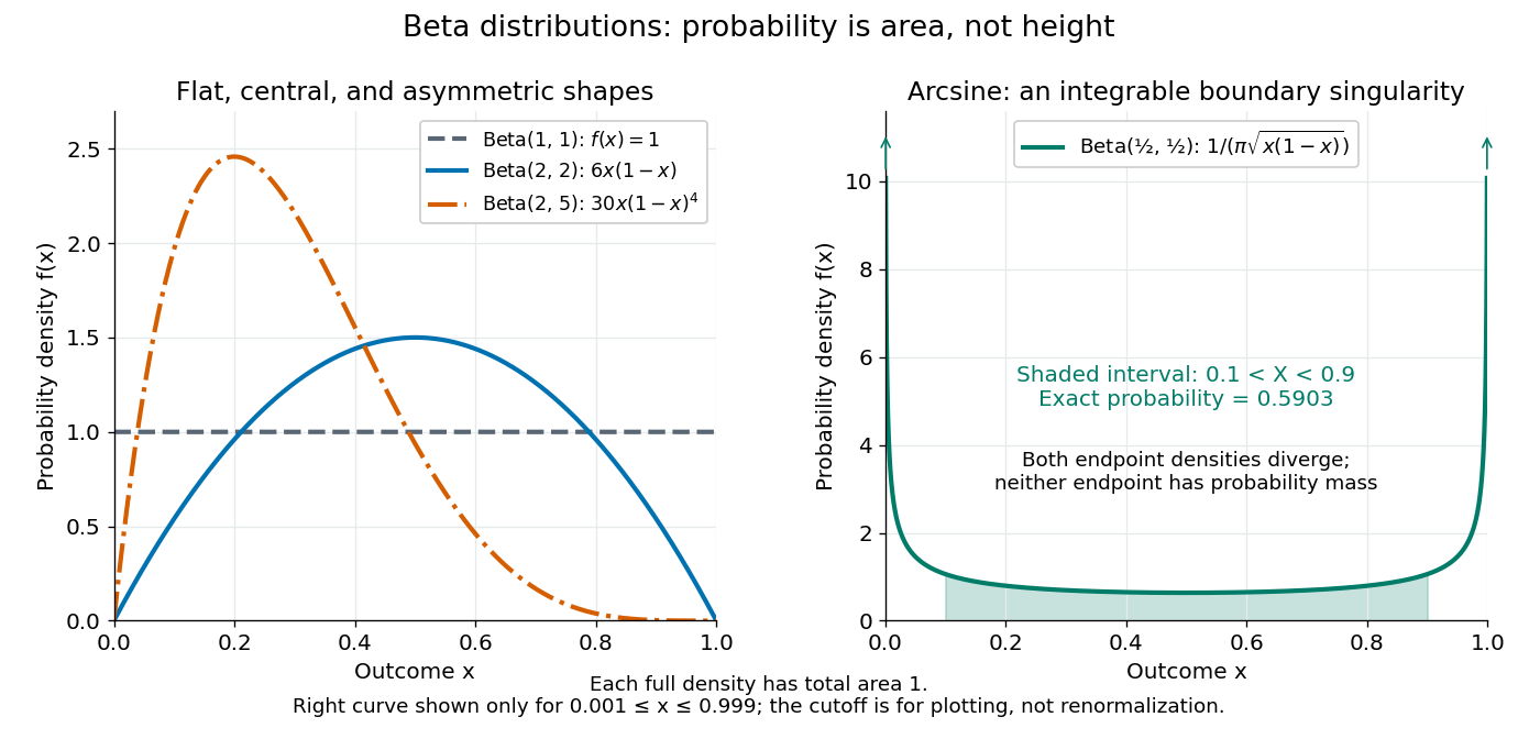
The arcsine distribution curve is plotted only for ; its finite plotted ends do not represent finite endpoint values of the probability density function. Using the inverse sine, the shaded central interval has exact probability , calculated analytically rather than by treating the cropped curve as normalized.
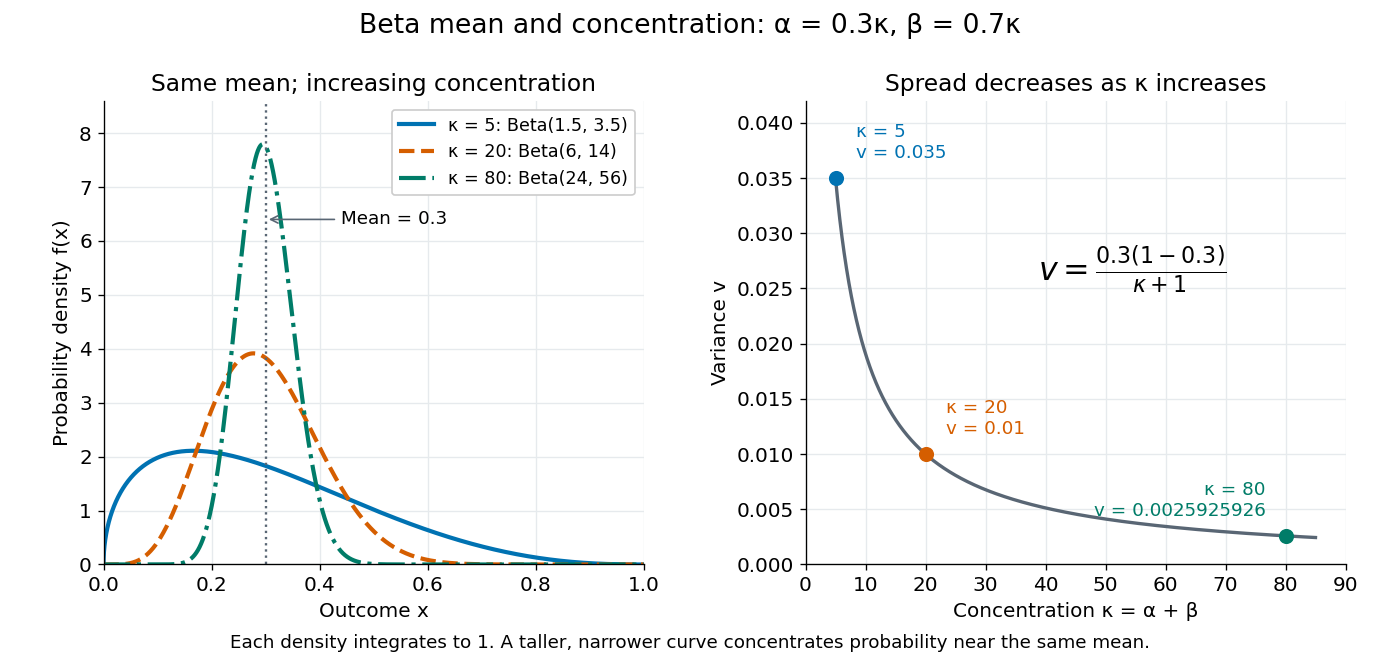
To separate location from spread, write and . The mean and variance of the beta distribution areThe mean specifies the balance between the parameters; their sum controls concentration about that mean. Multiplying both parameters by the same positive number preserves the mean and changes the variance. Larger puts more area near and makes the probability density function taller there; the total area stays one. Small allows much greater spread, sometimes favoring the endpoints rather than the mean itself.
For example, keeping mean and taking gives the beta distributions , , and . Their variances are , , and , respectively. Parameters need not be integers.


The formulas follow from two short moment calculations. Multiplying the probability density function by or increases the first parameter of the Euler beta function:Apply the Gamma function recurrence to the beta--gamma identity, then subtract from to obtain the variance.
The beta distribution is especially convenient as a prior distribution for the unknown success probability of Bernoulli trials. The Beta-binomial conjugacy says that successes and failures update a prior distribution to a posterior distribution . For example, suppose a coin has prior distribution and we observe eight heads and two tails. Its posterior distribution is then , with posterior mean . [ref]
https://ocw.mit.edu/courses/18-05-introduction-to-probability-and-statistics-spring-2022/mit18_05_s22_class15-prep.pdf. MIT 18.05, Reading 15: beta priors and conjugate updating
.A truncated distribution is a conditional probability distribution obtained by restricting a random variable to a specified subset of its original support and renormalizing.
For a wavefunction satisfying the Schrödinger equation with a real potential,This continuity equation expresses local conservation of probability.
The Born rule connects a quantum state to measurement probabilities. Let be a complete orthonormal basis, finite or countably infinite, for a Hilbert space, and letAn ideal measurement distinguishing these basis vectors returns label with probabilityThis assignment is a physical measurement rule. Its compatibility with total probability one follows from orthonormality and normalization:The probabilities are the squared moduli, not the amplitudes themselves or the squares . [ref].
If the basis is an eigenbasis of an observable, the reported numerical value is its eigenvalue. Several vectors can share one eigenvalue; the probability of that value is then the sum over the corresponding basis labels. More generally, a projective measurement with orthogonal projections assignsfor a pure state and a general density matrix , respectively. This also covers mixed states and degenerate eigenspaces. The Born rule determines outcome statistics; the ideal conditional state change is specified separately by the Lüders rule. See projective measurement for that formulation and its assumptions. [ref]
https://quantum.cloud.ibm.com/learning/en/courses/general-formulation-of-quantum-information/general-measurements/formulations-of-measurements. Watrous, IBM Quantum Learning, Mathematical formulations of measurements, Projective measurements
.For a worked example, take the normalized qubit quantum stateThe squared moduli add to . A computational-basis measurement, equivalently a measurement of the Pauli matrix, hasThese probabilities do not depend on the relative quantum phase . Now choose the Hadamard basiswhose vectors are eigenstates of the Pauli matrix, also used by the Pauli X gate. The new probability amplitudes and probabilities areBoth probabilities are nonnegative and their sum is one. The relative quantum phase becomes visible because the two probability amplitudes add before their squared modulus is taken:
- At , and .
- At , .
- At , and .
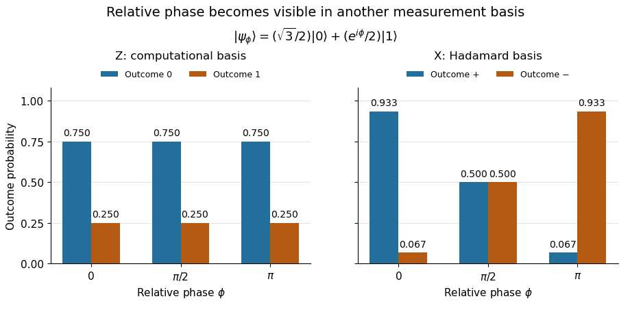
The same qubit preparation has phase-independent Z probabilities and phase-sensitive X probabilities
. Details. 
A Hadamard gate followed by a computational-basis measurement realizes these statistics, since , respectively. Compare the two bases using fresh, identically prepared copies: a preceding measurement may change the state. The quantum superposition section shows why replacing the preparation by the mixed state keeps the statistics but gives for every .
The usefulness of the Born rule is this conversion from linear algebra to experimental predictions: calculate overlaps in the basis actually measured, then take squared moduli. Its appealing geometry is that changing basis redistributes probability while preserving total squared norm. The same rule relates an energy eigenstate expansion to an energy measurement and a position wavefunction to a probability density.
Born's 1926 paper on quantum scattering interpreted the outgoing-wave coefficients in terms of the probabilities of collision outcomes; a corrective footnote specified proportionality to the square of the amplitude. This is a historical scattering formulation, rather than the general density matrix formula above. [ref]
https://doi.org/10.1007/BF01397477. Born, Zur Quantenmechanik der Stoßvorgänge, Zeitschrift für Physik 37, 863–867, 1926
; [ref]https://www.neo-classical-physics.info/uploads/3/0/6/5/3065888/born_-_qm_for_collisions_i.pdf. English translation of Born's paper, p. 3 and footnote 1
.If a graph has minimum degree , then its graph Ramsey number satisfies . The probabilistic proof chooses a red-blue edge colouring and applies the local lemma to its monochromatic copies of .
There are unlisted articles, also show them or only show them.