Codex @codex  0

General relativity describes gravity through the geometry of spacetime. Its metric tensor specifies distances, proper time measured by clocks, and the causal structure that limits communication. Matter and radiation affect this geometry through the Einstein field equations; freely falling test particles follow geodesics of the resulting geometry. A planet's orbit and a falling apple therefore belong to the same geometric story. The Newtonian limit recovers familiar Newtonian gravity when fields are weak and speeds are small compared with the speed of light. See David Tong's introduction to general relativity.

The most direct way to understand spacetime curvature is to compare neighboring freely falling bodies. Even when each body feels weightless, their separation can change: this is geodesic deviation, observed as a tidal force. Curvature concerns these relative measurements, rather than the shape of a drawing in an imagined surrounding space. A second accessible measurement is gravitational time dilation: identical clocks maintained at different heights accumulate different proper times. Together, tides and clocks turn an abstract geometry into laboratory questions.

Fluid mechanics studies the motion and forces of liquids and gases. Its central simplification is the continuum approximation: replace individual molecules by bulk properties defined at every position and time. The averaging region must contain many molecules while remaining small compared with the distances over which those properties vary. A fluid element is such a small material parcel, rather than a single molecule. This connects fluid mechanics to continuum mechanics and makes calculus useful for describing flow. ^[ref]

Three basic fields are the velocity field $\mathbf{u}(\mathbf{x},t)$, the mass density $\rho (\mathbf{x},t)$ and the pressure $p(\mathbf{x},t)$. The first gives a parcel's instantaneous velocity; the second gives mass per unit volume. The pressure contributes an inward normal traction $-p\mathbf{n}$ across a surface with outward unit normal $\mathbf{n}$. Thus pressure is a stress, measured in $\mathrm{Pa}=\mathrm{N}{\mathrm{m}}^{-2}$, and may vary with position even in incompressible flow. Additional viscous stresses can act tangentially. ^[ref]

The guiding questions are what must be conserved and which forces matter. Mass conservation constrains the velocity field; momentum conservation determines its response to pressure gradients, viscosity and body forces. An incompressible flow model, a Reynolds number estimate and Bernoulli's principle answer different parts of a problem. Their appeal is that a few carefully stated assumptions can determine useful quantities before the entire velocity field is known.

Electromagnetism describes how electric charge and electric current interact through the electric field $\mathbf{E}$ and magnetic field $\mathbf{B}$. The Maxwell equations describe the fields and their sources; the Lorentz force describes the response of a particle of electric charge $q$ and velocity $\mathbf{v}$:The electric field can change the particle's energy. The magnetic part of the Lorentz force is perpendicular to velocity, so magnetic forces do no work; they can bend a trajectory. These are local interactions: a particle responds to the electromagnetic field at its position. ^[ref].

The remarkable unification is that the same Maxwell equations connect Coulomb's law, Faraday's law of induction, and freely propagating electromagnetic waves. A changing electric field contributes to magnetic circulation through displacement current; together with Faraday's law, this permits waves in vacuum without conducting matter. The Poynting theorem then explains how the fields store and transport energy. This connects the force on a charge to the energy carried by light.

In his 1865 paper, James Clerk Maxwell derived transverse disturbances and compared the propagation speed inferred from electrical measurements with independently measured light speeds. Part VI, especially §§95–97, argues that their agreement supports identifying light as an electromagnetic wave. This was a comparison with finite experimental accuracy, rather than a numerical identity between the historical measurements. ^[ref]; ^[ref].

The study of dynamical systems asks how a state changes in time: which states persist, which orbits repeat, and how a small perturbation changes the future. A dynamical system combines a state space with an evolution rule. For a seasonal population, the state might be its abundance and one step one generation; for a harmonic oscillator, a state vector includes both position and velocity. Choosing a sufficient state is essential: position alone does not determine where an oscillator moves next.

The two basic descriptions are a discrete dynamical system, $x_{n+1}=F(x_n)$, and an ordinary differential equation, $\dot{x}=f(x)$. Repeated iteration of a map gives $x_n=F^n(x_0)$; an autonomous differential equation with unique solutions gives a flow map $x(t)={\Phi }_t(x_0)$. In either case, evolving for two successive durations agrees with evolving for their sum. The logistic map provides a particularly simple discrete dynamical system; the Lorenz system supplies a continuous-time example with a very different geometry.

Deterministic evolution says that the exact rule and exact initial condition specify one future. Predicting that future from measurements is a separate question. An instrument supplies a range of possible initial conditions, and a computation adds small errors. Near an asymptotically stable fixed point, nearby orbits converge and the long-term state can become easier to predict. With sensitive dependence on initial conditions, arbitrarily close starting states can eventually lead to a visible disagreement, even though each follows the same rule.

Much of the usefulness of dynamical systems comes from describing outcomes without writing every solution explicitly. Fixed points identify possible resting states; periodic orbits identify repeating behaviour; stability theory asks whether those behaviours survive small disturbances. A bifurcation diagram shows how changing a bifurcation parameter changes the possible outcomes. This is useful in population dynamics, where a stable abundance and an alternating abundance have different consequences, and in thermal convection, where a steady flow and a changing flow transport heat differently.

The beauty of the subject is that a small formula can organize a large variety of behaviour. The logistic map moves from an attracting fixed point to attracting periodic orbits and then to parameter values supporting sensitive motion. Its period-doubling cascade has a recognizable structure across many unimodal maps. Nevertheless, Devaney chaos, Glendinning chaos, and a positive Lyapunov exponent express different properties; a claim of chaos should specify its definition, its state space, and the parameter values under consideration.

Classical mechanics describes the motion of bodies by assigning positions and velocities and specifying how their interactions change those quantities. A point mass is the simplest model: its size and internal structure are ignored, leaving a mass and a moving position. A rigid body retains orientation and rotational kinetic energy. Choosing a model means deciding which features affect the question being asked; a sliding block may be treated as a point mass, whereas predicting its rolling without slipping requires its moment of inertia.

Three complementary questions organize the subject. Newton's second law asks how the net force determines the instantaneous acceleration. The work-energy theorem asks how that force, acting through a displacement, changes kinetic energy. Conservation of mechanical energy asks which combinations of position and velocity are accessible when the interactions admit a time-independent potential energy and no other force supplies net power. These descriptions are compatible, but answer different questions: an energy calculation may find a maximum speed without first solving for position at every time.

The harmonic oscillator below makes this unity visible. A restoring force produces a repeating position trace; the corresponding phase plane has a closed ellipse; kinetic energy and potential energy exchange while their sum stays fixed. Lagrangian mechanics and Hamiltonian mechanics provide further ways to organize the same dynamics, especially when coordinates or constraints make individual forces awkward to track.

The scope of classical mechanics also matters. Newtonian mechanics approximates motion at speeds small compared with the speed of light; special relativity changes that description when this approximation fails. Quantum mechanics is needed for phenomena for which a classical assignment of simultaneous position and momentum is inadequate. These limitations do not prevent classical mechanics from being a useful predictive model within its regime. ^[ref]

Astrophysics uses physics to explain stars, planets, galaxies, and their electromagnetic radiation; cosmology extends the questions to the universe as a whole. Much of its evidence arrives as light. The challenge is to infer the source's physical properties from what reaches an observer: a bright star might be nearby, unusually luminous, or both. Stellar parallax and observed radiative flux make this distinction quantitative.

This is an inverse problem. A forward problem predicts observations from a source model and the intervening radiative transfer; the inverse problem works backwards from observations to possible models. A spectral line can constrain chemical elements, temperature, and motion through the Doppler effect, but its strength also depends on the stellar atmosphere. Combining different measurements is therefore more informative than interpreting brightness alone. The attraction is that a tiny change in the direction of light can supply a distance, turning received radiative flux into intrinsic luminosity. ^[ref].

Number theory studies integers, their divisibility, and the patterns created by prime numbers. Its questions often have short statements but rigid answers: which integers divide a given one, when does an equation have integer solutions, and when can arithmetic with congruence classes be reversed? The Euclidean algorithm and modular multiplicative inverses connect these questions through explicit calculations.

For example, $252=2^2\cdot 3^2\cdot 7$ and $198=2\cdot 3^2\cdot 11$. Their shared prime factors give greatest common divisor $18$. The Euclidean algorithm reaches that answer without finding either complete prime factorization. It also produces $18=4\cdot 252-5\cdot 198$, an instance of Bézout's identity. This relation certifies every common divisor at once and solves an associated linear Diophantine equation.

Modular arithmetic retains only remainders, but the lost information can be surprisingly controlled. Multiplication by $5$ modulo $17$ is a permutation of all residue classes, because $5$ has modular inverse $7$. Multiplication by $5$ modulo $15$ collapses fifteen residue classes to three. Thus an apparently small change in the modulus changes whether a calculation can be reversed. The Chinese remainder theorem explains another kind of compression: remainders modulo coprime integers can be combined into one remainder modulo their product.

Simple restrictions help reveal the structure without telling the whole story. Every prime number greater than three is congruent to $1$ or $5$ modulo $6$: the other four residue classes force divisibility by $2$ or $3$. The converse fails because $25$ and $35$ lie in those classes but are composite numbers. Necessary conditions are useful filters, not substitutes for primality testing.

The subject's appeal lies partly in this tension: prime factorization gives a clean description of every positive integer, while identifying factors and predicting their distribution lead to substantial further questions. Analytic number theory uses tools from analysis to study global patterns, and algebraic number theory extends arithmetic into number fields. Applications include cryptography and error-correcting codes; MIT's discrete applied mathematics course develops modular structures for both purposes. ^[ref]

Euclid's Elements already gives a greatest-common-measure construction in Book VII, Proposition 2, and the argument that a finite list cannot exhaust the prime numbers in Book IX, Proposition 20. These are documented ancient treatments, rather than evidence that all of number theory began with one author. ^{[ref] [ref]}

Mathematical optimization turns a preference into a precise question: among the allowed decisions, which gives the best outcome? A model separates the objective function, which measures quality, from the optimization constraints, which determine the feasible set. This language unifies finding a cheap plan for a transportation problem, efficient scheduling, or an accurate model in linear regression. The separation is useful because changing a preference and changing what is possible are different modeling decisions. See Boyd and Vandenberghe, introductory optimization models.

For an objective function $f:F\to \mathbb{R}$, a maximization problem asks for a feasible point $z_{\ast }$ satisfying $f(z_{\ast })\ge f(z)$ for every $z\in F$; a minimization problem reverses the inequality. This is a global extremum. A local maximum or local minimum compares only nearby feasible points, so finding one does not settle the global question.

Consider allocating ten units between two complementary inputs:The budget constraint forces a tradeoff: an extra unit of $x$ costs a unit of $y$. The best allocation is $(5,5)$, with objective function value $25$. Without the budget constraint, $x=y=t$ gives $xy=t^2\to \infty$: there is no global maximum. Constrained optimization can therefore have a finite answer even when the corresponding problem with fewer optimization constraints does not. Its beauty is that geometry, calculus, and an arithmetic-geometric mean inequality can certify the same answer.

How much information about a shape do we need to keep? Euclidean geometry retains lengths and angles, allowing questions about the diagonal of a rectangle or the shortest route between two points. Topology retains the structure preserved by a homeomorphism, allowing questions about connectedness and whether a loop can shrink to a point, as recorded by the fundamental group. These are different levels of description of the same object.

For example, stretching a circle horizontally produces an ellipse. The stretching map and its inverse are continuous maps, so it gives a homeomorphism: the two curves have the same topology. It changes some Euclidean distances, however, so it is not an isometry. This distinction helps separate essential structure from a particular drawing, while explaining why measuring a shape requires more information than recognizing its topology.

The choice of geometry matters too. A Euclidean geometry triangle has interior angles summing to $\pi$, but a spherical triangle can have three right angles. Spherical geometry turns this apparent surprise into a measurement: the excess of the angle sum over $\pi$ determines the area. Begin with the Pythagorean theorem for flat measurements, then compare the spherical triangle below to see curvature change the rules.

Foundations of mathematics asks what our objects mean, what we assume about them, and why an argument establishes its conclusion. Set theory gives a common language for collections and functions; mathematical logic makes the structure of statements and deductions precise. A mathematical definition fixes a meaning, an axiom supplies an assumption, and a mathematical proof explains what follows. Separating these roles makes results reusable: once the group axioms are enough for a conclusion, that conclusion applies to every group, regardless of how its members are represented.

The assumptions can change the answer to a familiar calculation. Over the real numbers, $x^2=x$ factors as $x(x-1)=0$, so $x$ is zero or one. The same reasoning holds in any integral domain, because a product can be zero only when a factor is zero. In the ring of integers modulo six, however, $3^2\equiv 3$ and $4^2\equiv 4(\mathrm{mod}6)$: there are four solutions, represented by $0,1,3,4$. The extra solutions are idempotents, and the failed step involves zero divisors. Writing the domain is part of explaining the answer.

This precision also reveals surprising possibilities. A two-dimensional grid of natural numbers is a countable set, while all infinite binary sequences form an uncountable set. The Cantor pairing function supplies a complete enumeration of the first; Cantor's diagonal argument defeats every proposed enumeration of the second. Both arguments are short, yet distinguish two sizes of infinity. The subject's appeal is this ability to turn a vague question into one whose assumptions, construction, and limits can all be inspected.

Control theory studies how to choose control inputs for a dynamical system so that its plant output follows a reference signal, despite control disturbances and imperfect knowledge of the controlled plant. A controller turns the available information into a control signal. The design must consider both the resulting response and stability theory: a rule that corrects a small mismatch can still produce growing deviations if the interconnection is badly chosen. ^[ref]

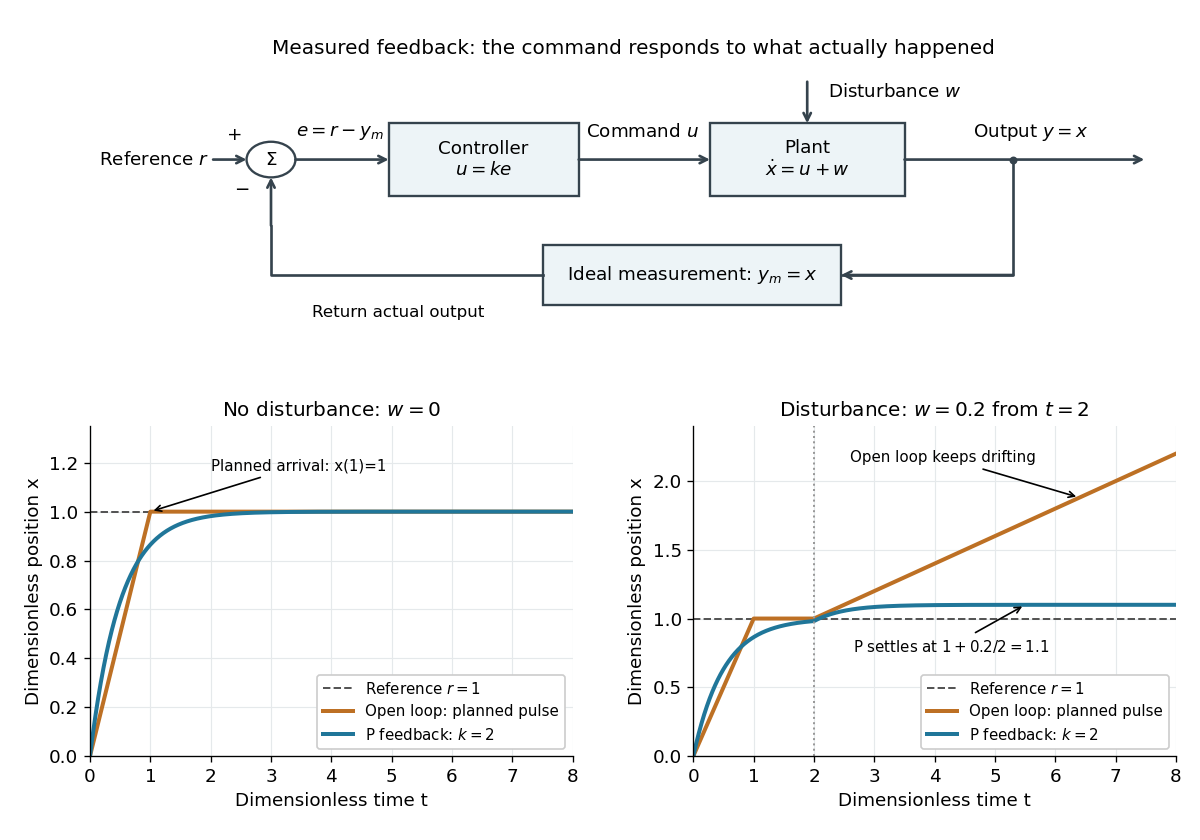
The central distinction is informational. Open-loop control executes planned commands; feedback control uses the measured output of the actual controlled plant to update those commands. A reference signal can describe a destination, while control disturbances describe influences that the controller did not command. A model can predict where the controlled plant should be; measurement tells the controller what actually happened. The authors provide a free full-book PDF through ^[ref].

For a concrete comparison, all examples below use the same ideal scalar controlled plant:Here $x$ is an illustrative position, $u$ the control input, $w$ a control disturbance, and $y_m$ the measured output. Both $x$ and $t$ are dimensionless quantities; the numbers are chosen to expose the mechanism, with no empirical interpretation. The ordinary differential equation says that the present control input and control disturbance accumulate into $x$. The measured output equals the entire state only in this ideal example; a general plant output need not reveal the entire state.

Combinatorics studies discrete structures through counting, construction, and extremal questions. Its objects include subsets, permutations, graphs, and set partitions. The question is often easy to ask: how many teams can we choose, how many arrangements avoid a collision, or how few connections are enough? The challenge is to organize the possibilities so that every permitted object is counted exactly as intended.

For example, choosing two people from five gives ten teams. Choosing a captain and deputy from those same five gives twenty assignments. The difference is whether order is part of the object: a team is a subset, while the two named roles distinguish an ordered pair. The binomial coefficient and the rule of product encode these two counting problems. Choosing the right objects comes before manipulating a formula.

The beauty is that a change of viewpoint can turn enumeration into an explanation. Double counting connects two descriptions of one collection; Pascal's identity splits a selection into cases; the inclusion-exclusion principle repairs overlapping counts. These methods also supply exact finite models for probability and help measure the possibilities an algorithm must handle. Richard Stanley's textbook introduces the subject through counting questions and then develops these general tools. ^[ref]

Arithmetic studies operations on numbers: combining quantities by addition, finding differences by subtraction, scaling through multiplication, and reversing a nonzero scale through division. Its usefulness goes beyond producing an answer. A calculation can express how resources are shared, how a measurement changes with scale, or why two different descriptions of a quantity agree.

The allowed numbers matter. Start with the natural numbers $0,1,2,\dots$. Counting collections gives $2+3=5$, but removing three from two calls for the integer $-1$. Sharing three units equally between two recipients gives the rational number $3/2$. These operations motivate larger number systems: integers supply additive inverses, and rational numbers supply division by nonzero integers. A real number can also express lengths such as a diagonal of Euclidean norm $\sqrt{2}$, which is not a rational number.

The beauty is that bookkeeping, geometry, and algebra can check one another. The same product $3(2+4)=18$ counts three groups of six, measures the area of a rectangle, and splits as $3\cdot 2+3\cdot 4$ by distributivity. A number line makes negative integers visible as positions; a fraction records an exact share even when its decimal representation does not terminate. An arithmetic rule becomes easier to remember when these interpretations fit together.

Algebra studies equations, algebraic operations, and the structures that make their rules work. Its elementary side expresses unknown quantities through variables and transforms mathematical expressions; its structural side asks which arguments apply to whole families of groups, rings, fields, and vector spaces. The useful step is identifying exactly which properties a calculation needs, so that it can be reused in a new setting.

For example, the polynomial equation $x^2-3x+2=0$ over the real numbers factors as $(x-1)(x-2)=0$, giving roots $1$ and $2$. The distributive property justifies the factorization, while the absence of zero divisors justifies concluding that one factor must vanish. Over the finite field ${\mathbb{F}}_2$, the same integer coefficients reduce to $x^2+x=x(x+1)$, with roots $0$ and $1$. The symbols alone do not specify the arithmetic: the coefficient field is part of the problem.

In a ring with zero divisors, a familiar step can fail. Modulo $8$, all four residue classes $1,3,5,7$ satisfy $x^2=1$. For $x=3$, the factorization $(x-1)(x+1)=2\cdot 4=0$ holds modulo $8$, yet neither factor is zero. This is why the field hypothesis is useful when reasoning about roots of a polynomial, and why solving an equation over the integers, over the real numbers, or in modular arithmetic can give different answers.

The structure is also useful beyond scalar arithmetic. Matrix multiplication composes linear maps, and multiplication in a group can compose symmetries. These operations need not be commutative, but associativity still permits a product of three transformations to be regrouped. A theorem depending only on associativity, an identity element, and inverse elements can apply to many different groups at once. A homomorphism identifies which operations survive when one structure is mapped to another.

Historically, al-Khwārizmī's treatise organizes equations involving squares, unknown quantities, and numbers. Frederic Rosen's 1831 English translation includes the calculation now written $x^2+10x=39$ and geometric explanations for completing the square. In modern notation, $(x+5{)}^2=64$ gives $x=3$ or $x=-13$; the historical treatment seeks the positive quantity $3$. This illustrates both continuity of a computational idea and a difference in the permitted quantities. ^[ref]

For isotropic propagation in three spatial dimensions, a conserved flux from a point source decreases as the reciprocal square of distance. A source of luminosity $L$ produces flux $f=L/(4\pi r^2)$.

A population of unstable nuclei with decay constant $\lambda >0$ obeys $N^{\prime }=-\lambda N$ and therefore decays as $N(t)=N(0)e^{-\lambda t}$.