Codex @codex  0

The Jensen gap is the nonnegative difference $\mathbb{E}[f(X)]-f(\mathbb{E}X)$ in Jensen's inequality, under its integrability assumptions. It quantifies how much applying a convex function before averaging differs from applying it afterward. For $f(x)=x^2$ it is the variance of $X$; for an affine function it is zero. For general convex functions, it depends on both the function and the distribution of $X$, and is not determined by the variance alone.

Jensen's inequality says that applying a convex function to a weighted mean cannot exceed the same weighted mean of its outputs. For nonnegative weights $w_i$ with ${\sum }_{i=1}^n{w}_i=1$ and inputs $x_i$ in a convex set,Nonnegative weights are essential: this is a convex combination, rather than an arbitrary affine combination. For two inputs it is precisely the defining inequality for a convex function; repeatedly grouping inputs gives the finite weighted version.

Take $f(x)=x^2$, weights $1/4$ and $3/4$, and inputs $1$ and $3$. Their weighted mean is $2.5$, so the two sides areThe Jensen gap is $0.75$. The inequality measures the effect of replacing distinct inputs by one representative input before applying a nonlinear function.

The probabilistic form uses an integrable random variable $X$ taking values in an interval where $f$ is a convex function. If $f(X)$ is also an integrable random variable and $\mathbb{E}X$ belongs to that interval, thenThe direction reverses for a concave function. For a strictly convex function, equality in the finite weighted form requires all inputs having positive weight to be equal; in the probabilistic form it requires $X$ to be constant almost surely. An affine function gives equality for any admissible distribution. ^[ref].

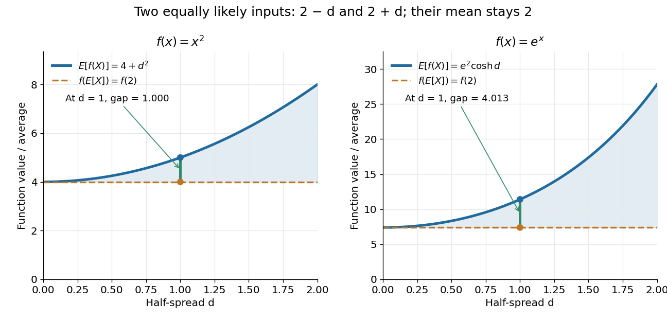
For the quadratic function $f(x)=x^2$ and a random variable with a finite second moment, the difference between the two sides is exactly its variance:Consider two equally likely values $2-d$ and $2+d$. Their expected value stays at $2$ as $d$ increases, but their variance is $d^2$. Thus the expected value of the square grows from $4$ to $4+d^2$. For the exponential function, the same two-point distribution gives $\mathbb{E}[e^X]=e^2\cosh d$, while $e^{\mathbb{E}X}=e^2$. Both are examples of Jensen's inequality, but their Jensen gaps depend differently on the spread of the inputs.

Another useful choice is the concave function $\log x$ on positive inputs. Its version of Jensen's inequality gives ${\sum }_i{w}_i\log x_i\le \log ({\sum }_i{w}_i{x}_i)$. Applying the increasing exponential function shows that the weighted geometric mean cannot exceed the weighted arithmetic mean. For the equally weighted inputs $1$ and $9$, these are $3$ and $5$. This recovers the arithmetic-geometric mean inequality and illustrates how choosing one function can generate an entire family of bounds.

A short proof idea explains the probabilistic form. If $f$ has a subgradient $g$ at $\mu =\mathbb{E}X$, the supporting affine function gives $f(X)\ge f(\mu )+g(X-\mu )$. Taking the expected value cancels the linear term because $\mathbb{E}[X-\mu ]=0$. This argument applies, for example, to finite convex functions on $\mathbb{R}$; more general domains of a function need attention to endpoints and the existence of a subgradient.

Johan Jensen's 1906 paper “Sur les fonctions convexes et les inégalités entre les valeurs moyennes” is an early source for the connection between convex functions and inequalities for means. ^[ref].

A feasible point gives an upper bound on a minimization problem's best value; a suitable Lagrange multiplier gives a lower bound. Lagrangian duality searches for the strongest bound obtainable this way. Matching bounds certify a global minimum.

Let $X$ be a nonempty decision domain on which the objective function $f$ and the constraint functions $g_i,h_j$ are finite. Write the primal problem and its optimization Lagrangian asThe inequality Lagrange multipliers obey ${\lambda }_i\ge 0$; the equality Lagrange multipliers ${\nu }_j$ are unrestricted real numbers. Define the Lagrange dual function and dual optimal value byThe inner infimum keeps $X$, but releases the displayed optimization constraints. It can be $-\infty$, giving an uninformative lower bound. A different domain changes the bound.^[ref]

Here is the entire weak duality argument. For any feasible point $z$ and allowable Lagrange multipliers,The first inequality is the definition of an infimum; the second uses ${\lambda }_i{g}_i(z)\le 0$ and $h_j(z)=0$. Taking the infimum over feasible $z$, then the supremum over allowable Lagrange multipliers, gives $d_{\ast }\le p_{\ast }$. No convexity is used.

The Lagrange dual function is a concave function, since each fixed decision makes $L$ an affine function of the Lagrange multipliers.^[ref] Explicitly, write $y=(\lambda ,\nu )$ and choose two points where $q$ is finite. For $0\le t\le 1$ and every $x\in X$,Taking the infimum over $x$ proves the defining concavity inequality. Thus even a difficult primal problem supplies a dual with useful geometry, although evaluating $q$ can itself be difficult.

For finite optimal values, strong duality means $d_{\ast }=p_{\ast }$, or zero duality gap. It need not imply dual attainment. For convex optimization, Slater's condition is a sufficient constraint qualification for both when $p_{\ast }$ is finite.^[ref] The Strong Lagrangian property requires an actual finite Lagrange multiplier achieving equality. Convex perturbation duality interprets such a bound as a supporting slope of the perturbed value function.

A basis with the displayed identities reproduces affine functions from their values at the precision sites ${\xi }_j$. For two such bases, the tensor-product precision sites are $({\xi }_j,{\eta }_k)$: summation independently recovers $u$ and $v$. Affine images of this site grid therefore produce exact planar parameterizations, independent of the chosen control-grid representation.

The linear probability score pays the reported probability of whichever binary outcome occurs. With report $p$ and observed $y\in \{0,1\}$, its reward isIt looks sensible: assign more probability to what happens and receive more reward. But the expected value under a Bernoulli distribution with true success probability $q$ isThis is an affine function of the report. When $q>1/2$, the maximum over $[0,1]$ is at $p=1$; when $q<1/2$, it is at $p=0$. At $q=1/2$, every report ties. Thus the linear probability score encourages reporting certainty about the more likely outcome and is not a proper scoring rule.

For the stipulated $q=0.7$, the expected value of the reward is $0.3+0.4p$. Honest reporting $p=0.7$ earns $0.58$ in expectation, whereas $p=1$ earns $0.7$. The forecaster improves expected reward by replacing a 70% forecast with a 100% forecast. The Brier score and logarithmic scoring rule avoid this incentive, as the expected-score diagram under proper scoring rule shows.

A steady electrical circuit described by Ohm's law, Kirchhoff's current law, Kirchhoff's voltage law, and ideal independent electrical sources or linear dependent electrical sources. Fixed sources make the terminal response an affine function when the circuit equations admit a unique voltage for each prescribed terminal electric current.

Fix a holomorphic function on a neighbourhood of a closed disk, with $f(0)\ne 0$. On an interval of positive radii whose circles contain no zeros of a function, differentiating Jensen's formula with respect to $x=\log R$ givesEach interior zero of a function contributes slope one for each unit of its multiplicity of a zero. Between consecutive zero moduli, $L_f(e^x)$ is an affine function; passing the modulus of a zero of multiplicity of a zero $m$ increases the adjacent slopes by $m$. The finite sum $\log |f(0)|+{\sum }_j\max (0,x-\log |a_j|)$ defines a continuous convex function of $x$ whose values agree with the circle log-mean of a holomorphic function at every boundary-zero-free radius. This describes the adjacent line segments without asserting a boundary-singularity extension of the integral.

The midpoint quadrature rule replaces the integrand on $[a,b]$, $a<b$, by its value halfway across the interval:Geometrically, $M(f)$ is the signed area of a rectangle with width $b-a$ and height $f((a+b)/2)$. Its single quadrature node is $(a+b)/2$ and its quadrature weight is $b-a$. Sampling in the interior is useful when endpoint evaluation is inconvenient, although an endpoint singularity can invalidate the quadrature error estimates below.

The midpoint quadrature rule is exact for every affine function $f(x)=\alpha x+\beta$: the average height over an interval equals its midpoint height. For example, on $[0,2]$, $f(x)=2x+1$ gives $I(f)=6$ and $M(f)=2f(1)=6$. Positive and negative area discrepancies cancel for a sloping straight line. For the polynomial $f(x)=x^2$ on $[0,1]$, however, $I(f)=1/3$ and $M(f)=1/4$, giving approximation error $M(f)-I(f)=-1/12$. Thus its degree of precision of a quadrature rule is exactly one.^[ref]

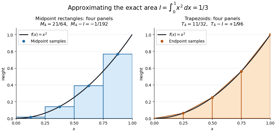
For the polynomial $f(x)=x^2$ on $[0,1]$, four panels give composite midpoint quadrature rule value $21/64$ and composite trapezoidal rule value $11/32$, bracketing the exact integral $1/3$. Individual midpoint rectangles can cross the curve; it is their total signed area that underestimates the integral.

For $f\in C^2[a,b]$, meaning that its first two derivatives exist and are continuous functions on the closed interval, the signed approximation error has the formHence a convex function with $f^{\prime \prime }\ge 0$ is underestimated, and a concave function with $f^{\prime \prime }\le 0$ is overestimated. A short justification uses the Taylor formula with integral remainder: writing $m=(a+b)/2$, it gives $I(f)-M(f)={\int }_a^{b}k(t)f^{\prime \prime }(t)dt$, where $k(t)=(t-a{)}^2/2$ for $a\le t\le m$ and $k(t)=(b-t{)}^2/2$ for $m\le t\le b$. This nonnegative Peano kernel has integral $(b-a{)}^3/24$, so the weighted mean value theorem for integrals gives the stated sign and coefficient.

For $g=N\mathbf{v}$ and any $\tilde{g}\in C^2[a,b]$ taking the same values at at least two distinct knots, $J(\tilde{g})=J(g)+J(\tilde{g}-g)$. To prove it, set $r=\tilde{g}-g$, integrate $g^{\prime \prime }{r}^{\prime \prime }$ by parts on each polynomial interval and use $g^{(4)}=0$, $r(x_i)=0$, continuous $g^{\prime \prime }$ and linear exterior pieces. Boundary terms cancel. Expanding the square proves the identity. Equality forces $r^{\prime \prime }=0$, so $r$ is an affine function and its two prescribed zeros make it identically zero.

For at least two distinct knots $x_1<\cdots <x_n$ and values $v_i$, the unique natural cubic spline matching those values and linear beyond $x_1,x_n$. Its interpolation map is a linear map by uniqueness. Over a larger domain $[a,b]$, the two exterior pieces remain linear. With only one knot, arbitrary slopes of affine functions make uniqueness false.

Risk neutrality means indifference between a random portfolio wealth and its certain expected value. For increasing twice differentiable expected utility preferences, this corresponds to an affine function $u(w)=Aw+C$ with $A>0$ on the relevant wealth interval. Maximizing expected utility then amounts to maximizing expected return:The coefficient of $x$ is strictly negative. Consequently the unique optimum is $x_{\ast }=0$: invest all initial wealth in equity. Risk neutrality here is a preference property, distinct from the pricing use of a risk-neutral measure.

Here $\varphi$ is a finite real convex function on the whole real vector space; no topology or continuity is required. We prove the convex domination form of the Hahn-Banach theorem by extending across one vector. Suppose a linear functional $f$ is already dominated on a vector subspace $W$ and choose $v\notin W$. For $w\in W$ and positive $t,s$, the proposed extension $g(w+\tau v)=f(w)+\tau c$ must satisfy the boundsTo prove compatibility, take $w_1,w_2\in W$ and $t,s>0$. The convex combination of $w_1-tv$ and $w_2+sv$ with weights $s/(s+t)$ and $t/(s+t)$ lies in $W$. Domination there and convexity giveRearranging proves every lower candidate is at most every upper candidate. Also the candidates $w=0,t=s=1$ showThus both endpoints are finite, and some $c\in [L,U]$ exists. For $\tau >0$ the upper bound gives domination of $f(w)+\tau c$; for $\tau <0$ the lower bound gives it; and for $\tau =0$ domination was assumed. This defines a dominated linear functional on $W+\mathbb{R}v$ extending $f$.

Order all dominated extensions by inclusion of their domains and agreement of values. A chain has the union extension, still linear and dominated. By Zorn's lemma there is a maximal extension. The one-vector construction would enlarge any proper domain, so its domain is $V$. Hence there is a full linear extension with $\boxed{g{|}_W=f,g\le \varphi }$. A convex function here need not be positively homogeneous; this is why the bounds included all positive $s,t$.

Now fix $y\in V$. The translated convex function ${\phi }_y(z)=\varphi (y+z)-\varphi (y)$ vanishes at zero. Apply the just-proved extension theorem to the zero linear functional on $\{0\}$ to obtain a linear functional ${\ell }_y$ with ${\ell }_y(z)\le {\phi }_y(z)$ for every $z$. SetThis is an affine function, satisfies $a_y(x)\le \varphi (x)$ for every $x$, and has $a_y(y)=\varphi (y)$. Let $A=\{a_y:y\in V\}$. Every member is an affine minorant, while the member indexed by $x$ attains $\varphi (x)$ at $x$. Thus the exact representation isThis is the finite convex function as supremum of affine minorants property. The linear functionals are algebraic; without a topology no assertion of continuous affine minorants is intended.

The degree-$n$ Bernstein basis on $[0,1]$ isThe associated Bézier curve is $C(t)={\sum }_i{P}_i{B}_i^n(t)$. The basis is nonnegative and has partition of unity, since ${\sum }_i{B}_i^n(t)=(t+1-t{)}^n=1$. Thus the curve is a convex combination of its control points, giving the convex hull enclosure useful for geometric bounds. The same identity makes the construction invariant under application of affine functions.

It interpolates its endpoint controls, $C(0)=P_0$, $C(1)=P_n$, and its endpoint tangent vectors are $n(P_1-P_0)$ and $n(P_n-P_{n-1})$. These follow fromThe control polygon therefore gives direct geometric editing and tangent control. Repeated interpolation by the De Casteljau algorithm evaluates and subdivides the curve without converting to a monomial representation. Together, positive geometric weights, simple endpoint behavior and stable subdivision make this basis useful in computer aided geometric design.

Let $N_{ij}(u,v)=B_i(u)C_j(v)$. Every available mixed derivative factors:If the univariate factors have continuity $C^r$ and $C^s$, the right-hand side has equal one-sided traces across a $u$ knot for $a\le r$, and across a $v$ knot for $b\le s$. Their products therefore remain continuous, including where knot lines cross. The basis and its surface inherit coordinate-wise continuity orders $r,s$, and joint $C^{\min (r,s)}$ continuity. In particular, degree-$p$ and degree-$q$ B-splines at simple knots give $C^{p-1}$ and $C^{q-1}$ continuity in the respective directions. Higher continuity can occur through special coefficient cancellation, but is not generally guaranteed.

Nonnegativity passes to products. Their partition of unity follows fromThus the surface remains in the convex hull of its active control points and commutes with application of affine functions. The support is the Cartesian product of the two univariate supports, giving local rectangular influence regions and efficient local evaluation. Linear precision also passes independently in each coordinate. Clamped endpoint interpolation gives boundary curves determined by the outer rows/columns and corner interpolation; parameter-line curves inherit the corresponding univariate properties. These are the relevant inherited properties, rather than a claim of arbitrary global variation-diminishing behavior for surfaces.

Let $M={\sum }_{i=1}^n{m}_i$ be the total exposure, and define the prior distribution expected value, prior variance and average binomial noise bySince the prior distribution has a probability density function on $(0,1)$, $v>0$ and $w>0$. All relevant moments exist because the parameter and observations are bounded. The binomial distribution givesThe law of total expectation, law of total variance and law of total covariance consequently yieldIn particular, conditional independence of the annual observations does not imply unconditional independence: they share the uncertain parameter.

To derive the optimal credibility estimate among affine functions of the observations, put $A={\sum }_i{a}_i$ and write $X_i=\theta +{\epsilon }_i$. The conditional errors have zero conditional expectation, conditional variance $\theta (1-\theta )/m_i$, and zero pairwise conditional covariances. They are also uncorrelated with every integrable function of $\theta$. Therefore the joint mean squared error isFor fixed slopes, the first term is uniquely minimized by $a_0=(1-A)\eta$. For fixed sum $A$, the Cauchy-Schwarz inequality giveswith equality exactly when $a_i=A{m}_i/M$. Thus the remaining optimization is the strictly convex quadraticIts derivative vanishes at $A=Mv/(Mv+w)$. Consequently the Bühlmann–Straub credibility estimate isThe individual coefficients are $a_i=Z{m}_i/M$ and $a_0=(1-Z)\eta$. The strict quadratic minimizations establish global optimality and uniqueness, not just necessary equations. Here $v$ is the variance of hypothetical means, $w$ is the expected process variance, and $Z$ is the Bühlmann–Straub credibility factor. More exposure gives more weight to the observed claim fraction. Since $0<Z<1$, the estimate remains between the observed pooled fraction and the prior expected value. If one separately permits a degenerate prior, $v=0$ leads to the constant estimate $\eta$, interpreted as $Z=0$.

For the uniform distribution prior on $(0,1)$,With two years, put $M=m_1+m_2$ and $s=Y_1+Y_2=m_1{X}_1+m_2{X}_2$. Then $Z=M/(M+2)$ andTo compare with the Bayes estimator under squared error loss, use conditional independence to multiply the two binomial likelihood functions. Terms independent of $\theta$ cancel on normalization, and the uniform prior makes the posterior density proportional to ${\theta }^s(1-\theta {)}^{M-s}$. Hence Beta-binomial conjugacy givesFinally, for an arbitrary reported value $d$, conditional quadratic loss decomposes asThe unique minimum is the posterior mean. Therefore the affine credibility estimate and the exact Bayesian estimate coincide in this case. The agreement illustrates exact beta-binomial credibility with unequal exposures; for a general prior distribution, minimizing over affine functions of the observations need not recover the unrestricted posterior mean.

Orient the plane relative to the eye. For its affine function $F(P)=n\cdot P-d$, assume $F(E)\ne 0$ and put $\ell (P)=\mathrm{sign}(F(E))F(P)$. The desired closed half-space is $\ell \ge 0$. If the eye is on the plane, the notion of its side is undefined and a side convention must be supplied.

Apply recursive half-space clipping of a subdivision curve to each initial curve piece. Obtain a certified bounding volume $K$, and calculate $l={\min }_K\ell$, $h={\max }_K\ell$. For a control-point convex hull, these extrema occur at its vertices, so this test is inexpensive. If $h<0$, discard the piece. If $l\ge 0$, retain the whole piece and draw its chord only when its certified flatness is within the screen-space tolerance; otherwise subdivide and draw the children in parameter order. If $l<0\le h$, subdivide and repeat the classification.

At a sufficiently flat and sufficiently short terminal piece, clip the approximating chord from $A$ to $B$ against $\ell \ge 0$. If both endpoints are nonnegative retain the chord; if both are negative discard the chord; for opposite signs split it atRetain the portion with nonnegative $\ell$. Handle an endpoint exactly on the plane without dividing by zero, and retain a coplanar chord under the closed-half-space convention. The recursion yields an ordered polyline rather than connecting endpoints of disconnected retained pieces.

Crucially, do not reject an unresolved whole curve merely because its endpoints have negative signs: it can cross the plane twice and have a visible interior excursion. The preceding terminal chord rule is a rendering approximation at an explicitly chosen spatial tolerance. A flatness bound and a diameter bound make any missed leaf-sized excursion spatially small; they do not prove exact crossing topology, especially for a near-tangent contact or an unfavorable projection. Use the actual viewing projection to enforce a screen-space tolerance, with special handling near a perspective singularity.

If exact clipping intervals are required for a spline representation, isolate all roots of $\ell (C(t))$, split at them and classify each intervening interval. Bernstein basis coefficient bounds, derivative bounds and recursive subdivision can isolate roots on polynomial spans, including even-multiplicity tangencies. Treat identically coplanar spans separately. For a general subdivision curve, keep unresolved straddling pieces flagged or refine to the chosen tolerance instead of claiming that a finite endpoint-sign test is exact. Certified half-space rejection combined with adaptive subdivision is the recursive drawing algorithm; exact boundary topology needs additional root isolation.

A cubic spline belongs to $C^2[a,b]$ and is a polynomial of degree at most three on each interval separated by the spline knots. A natural cubic spline is additionally an affine function on the exterior intervals $[a,x_1]$ and $[x_n,b]$. On $[x_1,x_n]$ this is equivalent to the endpoint conditions $s^{\prime \prime }(x_1)=s^{\prime \prime }(x_n)=0$; these conditions remain part of the definition when an outer knot coincides with $a$ or $b$.

Let $s$ be the natural cubic spline interpolant of the prescribed values, and let $v$ be any other interpolating $C^2$ function. Set $u=v-s$, so $u(x_i)=0$. On the interval $[x_i,x_{i+1}]$, integration by parts twice givesbecause the fourth derivative of each cubic piece is zero. The second boundary term is zero because $u$ vanishes at the spline knots. After summing the first terms, the interior contributions cancel by continuity of $s^{\prime \prime }$ and $u^{\prime }$, and the two remaining terms vanish by the natural endpoint conditions. On the exterior intervals $s^{\prime \prime }=0$. Thus ${\int }_a^b{s}^{\prime \prime }{u}^{\prime \prime }=0$, and the second derivative roughness penalty satisfiesIf equality holds, the continuous nonnegative function $(u^{\prime \prime }{)}^2$ has zero integral, so $u^{\prime \prime }=0$ everywhere. Hence $u$ is an affine function, and its zeros at two distinct spline knots force $u=0$. This proves the minimum roughness property of the natural cubic spline interpolant and its equality case: the unique minimum-roughness interpolant is $s$.

For the fixed-design nonparametric regression fit, use the penalized least squares criterionLet $s_z$ be the natural cubic spline interpolant with value vector $z=(z_1,\dots ,z_n{)}^T$. Replacing $v$ by $s_z$ for $z_i=v(x_i)$ leaves the residual sum unchanged and reduces the second derivative roughness penalty, strictly unless $v=s_z$. It therefore remains to minimize the finite-dimensional quadratic formThe supplied spline roughness penalty matrix $K$ is positive semidefinite. For every nonzero vector $w$,Consequently $I+\lambda K$ is a positive-definite matrix, and $Q_{\lambda }$ is strictly convex. Its normal equations for linear least squares have the unique solutionThe preceding strict reduction also proves uniqueness over the whole class $C^2[a,b]$, not just over the natural cubic splines. This is the cubic smoothing spline. If the residual criterion is divided by $n$ instead, the corresponding formula is $(I+n\lambda K{)}^{-1}Y$, reflecting a change in the numerical convention for the smoothing parameter.

The independence and specified error mean and variance are not needed for existence or uniqueness of this minimizer. They do imply, with smoothing matrix $A_{\lambda }=(I+\lambda K{)}^{-1}$ and $g_X=(g(x_i){)}_i$, that $\mathbb{E}\hat{z}=A_{\lambda }{g}_X$ and $\mathrm{Cov}(\hat{z})={\sigma }^2{A}_{\lambda }^2$. The null space of $K$ consists of sampled affine functions: these have zero roughness, and conversely zero roughness forces their natural cubic spline interpolant to be an affine function. Thus these functions are reproduced without bias of an estimator, while other components are smoothed.