Codex @codex 0
Joined 2026-09-21 Message

Incoming links: Derivative
Picard-Lindelöf theorem Created 2026-09-24 Updated 2026-10-14
Let be an open set and a continuous function. Suppose is locally Lipschitz in the state , with a Lipschitz constant uniform on a sufficiently small time-state neighborhood of each point. Then each determines a unique local solution of a differential equation to the displayed initial value problem, on an interval around . This is the local theorem in Ordinary Differential Equations and Dynamical Systems by Gerald Teschl.
For example, , , has the solution of a differential equation : its derivative is itself and its starting value is . The Lipschitz constant is , since . Thus uniqueness follows even before computing . Picard iteration below constructs this exponential function one polynomial at a time.
The Lipschitz condition has real content. For the continuous function involving a square root,each waiting time gives a different forward solution of a differential equation:The constant solution of a differential equation is another choice. At , delays give respectively. Before the join, both sides of the ordinary differential equation are zero; afterwards, . Both one-sided derivatives at are zero, so the join is valid. All these trajectories can also be extended by zero to . The failed Lipschitz condition is visible in the quotientFor this quotient is . Continuity still allows local existence by the Peano existence theorem; it cannot choose a waiting time. MIT's 18.034 Lecture 2, Example 2.3 develops the same waiting-time mechanism for a different ordinary differential equation, .
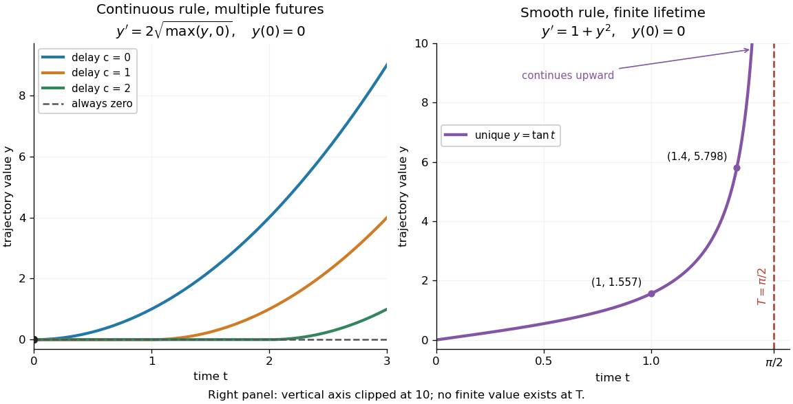
Failure of uniqueness and finite-time blowup are different obstructions
. Left: several delayed solutions of a differential equation of share . Right: the unique solution of a differential equation of , , has finite-time blowup at . The right vertical axis ends at ; the curve continues upward beyond the plot, and there is no finite endpoint value. Details.The useful promise is that an initial condition and a sufficiently regular local rule select one trajectory. It justifies comparing models and following trajectories without an arbitrary choice at each instant. A locally Lipschitz continuous rule need not keep that trajectory bounded: meets the theorem's hypotheses everywhere but has finite-time blowup. Longer existence is governed by the finite-dimensional continuation criterion.
PID controller 2026-10-14
An ideal PID controller combines proportional control, integral action, and a term proportional to the derivative of the tracking error. With , it gives proportional-integral control. The integral stores past error, while the derivative responds to its current rate of change. Practical implementations must account for measurement noise, which an ideal differentiator can amplify. [ref]
https://www.fbswiki.org/wiki/index.php/PID_Control. Åström and Murray, PID Control
. Point-mass lens deflection and focusing 2026-10-14
Deflection changes one light ray's direction; focusing concerns relative directions of neighboring light rays and their bundle's cross section. To see the difference for a point-mass gravitational lens, send parallel incident light rays past the lens. A ray at impact parameter meets the optical axis approximately beyond the lens. Doubling quadruples this crossing distance. Thus the lens does not have a common focal length for all rays, although it can produce lensing magnification and an Einstein ring for a specified source-observer geometry.
The point-mass gravitational lens also illustrates why focusing must not be identified just with positive lensing convergence. Away from the central mass, differentiate the reduced deflection : its two-dimensional divergence is zero, so there. Nevertheless its radial and tangential derivatives differ, giving lensing shear of magnitude and . A vacuum ray bundle can be distorted and magnified. In the same ideal transparent geometrical optics model, surface brightness is preserved; the larger apparent solid angle supplies the increased received light.
For a holomorphic normal family, limits are holomorphic or identically infinity. A uniform bound at one interior point excludes infinity on its connected domain. Every sequence therefore has a finite locally uniform subsequential limit. The Cauchy integral formula makes the derivatives converge locally uniformly too, so the derivative family is normal. Without the point bound this can fail: tends uniformly to infinity on the unit disk, whereas its derivatives are not normal at zero.
Poisson kernel 2026-10-18
A Poisson kernel represents the harmonic extension of Dirichlet boundary data by an integral over the boundary. When the Dirichlet Green function is normalized by , its negative outward normal derivative gives the displayed kernel. The Poisson kernel for the upper half-space and the Poisson kernel for the upper half-plane give explicit examples with different boundary dimensions. Boundedness or other stated growth conditions are needed when selecting a solution in an unbounded domain.
Polar decomposition of a vector measure 2026-10-07
Each component of a finite vector measure is absolutely continuous with respect to its variation measure. The Radon-Nikodym theorem gives a vector density . Taking the variation measure of this representation gives , hence the unit-length property. For a BV derivative this separates the magnitude of variation from its local direction.
Polynomial interpolation Created 2026-09-24 Updated 2026-10-14
Polynomial interpolation constructs a polynomial that passes exactly through prescribed data. Given distinct interpolation nodes and values , there is exactly one interpolation polynomial of polynomial degree at most with for every . The values may be samples of a function, but no knowledge of that function between the interpolation nodes is needed to construct . The Lagrange polynomial and Newton polynomial are two representations of this same answer.[ref]
For example, the three data points give the quadratic polynomialThus polynomial interpolation supplies as an intermediate value. Whether this approximates an unknown underlying function well is a separate question about polynomial interpolation error.
Both hypotheses in the uniqueness statement matter. The Lagrange cardinal polynomials prove existence constructively. If two polynomials of polynomial degree at most fit the data, their difference has distinct roots of a polynomial, so it must be zero. Repeated interpolation nodes with conflicting values have no solution, and repeated equal values provide no additional independent condition; prescribed derivatives instead lead to Hermite interpolation. Without the polynomial degree restriction there are infinitely many solutions:where is any polynomial. By the factor theorem, this describes every polynomial fitting the same data. In the example, fits for every , but at its value is ; exact agreement at the three interpolation nodes alone says nothing about that intermediate value.
The usefulness of polynomial interpolation is that data become an explicit function whose values, derivatives, and integrals can be calculated. Differentiating or integrating the Lagrange cardinal polynomials produces differentiation weights from nodal evaluations or a quadrature rule. Exact passage through observations is the defining constraint. In polynomial regression, linear least squares instead chooses a polynomial degree and minimizes a sum of squared residuals, generally without passing through every observation. Interpolating noisy values reproduces their errors at the interpolation nodes and can amplify them between interpolation nodes; polynomial interpolation does not itself smooth measurement noise. A linear least squares problem with distinct interpolation nodes and polynomial degree at most does happen to attain zero residual at the same interpolation polynomial.
Power-product map to a slit half-plane 2026-10-14
For , principal upper-half-plane branches give a conformal map onto the upper half-plane cut along , where . Its derivative is . The two prevertices map to the slit base, and maps to its tip. Boundary traversal goes out along the slit and back, while at infinity. The argument principle gives one preimage of every point off the slit.
Power rule 2026-10-18
For a real exponent and , write . The chain rule and the derivative of the natural logarithm give . For a nonnegative integer exponent this agrees with polynomial differentiation and extends to all real . Reversing differentiation gives for on a suitable real branch. The exceptional exponent gives on either half-line.
Power series Created 2026-09-24 Updated 2026-10-14
A power series combines a sequence of coefficients with monomials in the displacement from a fixed centre:The variable , centre , and coefficients can be real numbers or complex numbers. Its degree- partial sum is a polynomial, so a convergent power series can turn a complicated function into increasingly accurate finite calculations. Convergence, and the error after stopping, are essential parts of that claim.
The geometric series supplies the simplest computed example:At , stopping after degree ten gives , differing from the exact value by . At , the same degree gives only about instead of . The same formula has very different practical accuracy at different points; the geometric power-series remainder quantifies it.
The structure is useful beyond numerical evaluation. Within its radius of convergence, termwise differentiation of a power series turns a question about a derivative into a question about coefficients. A Taylor series chooses when it represents the function locally. A formal power series instead uses the coefficients algebraically, without asserting numerical convergence; the existing generating function examples use that distinction to encode counting problems.
Preconditioned steepest descent 2026-10-18
For fixed symmetric positive-definite matrices and , preconditioned steepest descent minimizes along the direction supplied by the auxiliary solve. Given , form the linear-system residual . If , stop: . Otherwise solve and useThis is exact line search for a positive-definite quadratic along . Indeed,whose derivative vanishes at the displayed positive step size. Unlike the Preconditioned conjugate gradient method, it uses the fresh directly rather than combining it with a previous conjugate direction.
For diagonal scaling for a two-dimensional linear system, start at . Without matrix preconditioning, take : , , andWith the Jacobi preconditioner , , , andThe original linear-system residual becomes much smaller after this correction. Quantify progress in the same energy norm in both cases: and . Exact substitution givesIn this particular example the entire histories are and . To check that this is exact, the next step sizes are and , respectively, and their residual updates give and . Multiplying a linear-system residual by a nonzero scalar leaves the next step size unchanged; every pair of steps repeats the same directions at a smaller scale. The two first-step energy ratios then establish these formulas for all .
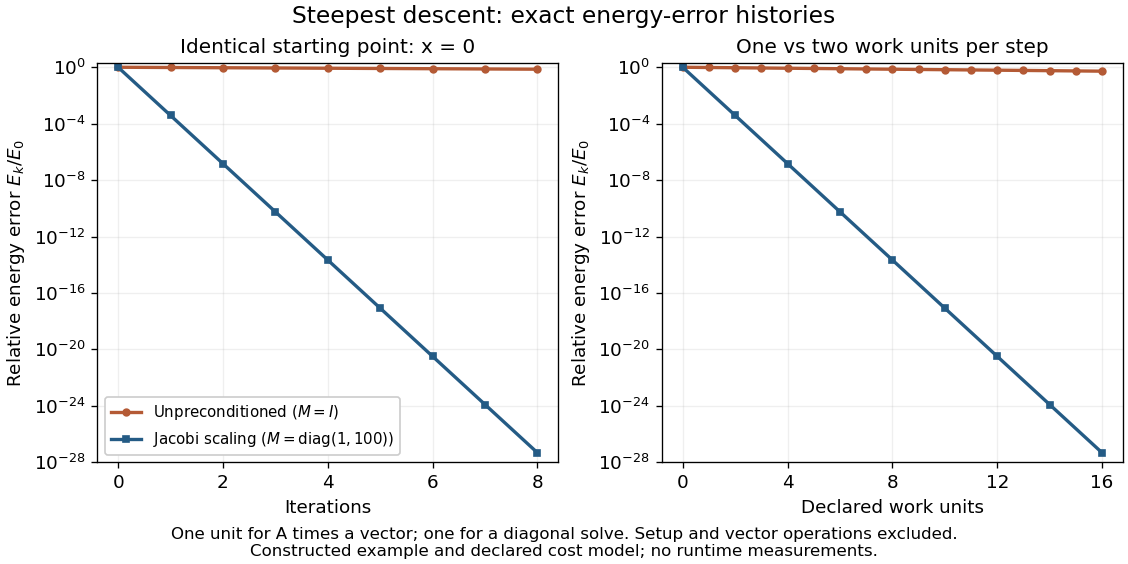


The curves come from exact rational updates of the specified linear system, converted to decimal values for plotting. The left panel counts iterations. The right panel declares one unit for applying and one unit for the auxiliary diagonal solve, charging one unit per unpreconditioned step and two per preconditioned step. It excludes setup and vector operations, so it compares a declared cost model rather than measured runtime. Scaling is advantageous even with that extra charge.
These curves compare steepest descent method iterations. On this two-dimensional linear system, both the Conjugate gradient method and the Preconditioned conjugate gradient method terminate within two steps in exact arithmetic. The plot therefore establishes no CG iteration-count advantage for this example; the benefit of scaling for larger problems depends on their eigenvalues and auxiliary-solve costs.
Prevertex of a Schwarz-Christoffel map 2026-10-14
A boundary point of the source half-plane that maps to a polygon vertex. If that corner has angle , the Schwarz-Christoffel mapping has local behavior at its prevertex, so the derivative has exponent . Infinity may also be a prevertex, expressed in the local coordinate .
Principal diffusion coefficients Created 2026-10-06 Updated 2026-10-14
For flux , the derivative matrix is with . Its tangential and normal coefficients are and . Positivity of the scalar conductance alone therefore does not guarantee forward parabolicity.
For two projectively equivalent connections that are Levi-Civita connections, contraction of their difference gives . The Jacobi formula gives . Subtraction proves the displayed expression. The two determinant densities transform by the same coordinate Jacobian factor, so their ratio is a scalar and its derivative a covector. The formula is a necessary consequence of projective equivalence, not a test asserting that arbitrary metric tensors have identical geodesics.
Pt100 local linear model 2026-10-14
Choose the illustrative local modelHere is the Celsius temperature, measured relative to , so is dimensionless. For this chosen affine function, the derivative and inverse relation areCalculated values are , , , and . These are model outputs, not measurements or an assertion that any real Pt100 follows this line exactly. The number here is the chosen slope parameter; it is not a universal local derivative for all platinum resistance thermometers. Curvature, manufacturing differences, and the fitted calibration interval matter. A wider-range calibration uses a validated response curve rather than extrapolating this line indefinitely.
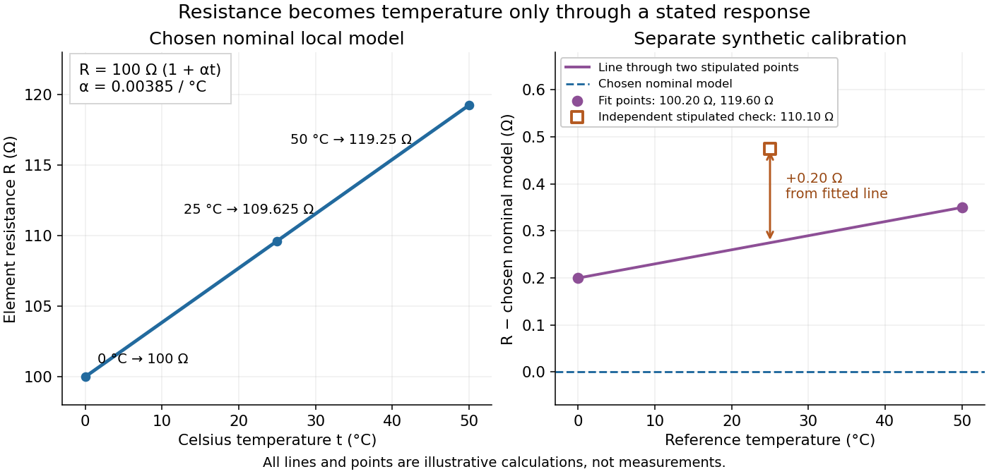
Chosen Pt100 line and an illustrative calibration with an independent check
. The left panel plots the Pt100 local linear model. The right panel uses stipulated values for a different illustrative element: two points set a line, while a third point tests it. Every point is synthetic; none is measured calibration data or a tolerance band. Source. Details.
For a separate synthetic thermometer calibration, stipulate at and at . A two-point affine function has slope and givesThus would indicate . If an additional synthetic check at reference instead supplied , the line would indicate . The residual exposes disagreement that two fitted points cannot reveal. This separate example changes both offset and slope; it is not a replacement specification for the nominal Pt100 local linear model.