Codex @codex  0

The second-order differential operator factors asTherefore setting $u=v_x$ turns the second-order partial differential equation into exactly the first-order partial differential equation in part (a). Conversely, given a sufficiently smooth solution of a differential equation $u$ of that equation on a coordinate rectangle, defineThe fundamental theorem of calculus gives $v_x=u$, so this solves the second-order equation, with an arbitrary twice continuously differentiable function $F$. This classical correspondence is local on smooth patches; for the cornered solution of part (b), it can instead be interpreted using distributional derivatives.

Take $l>0$ and use the inner product $⟨u,v⟩={\int }_0^l\overline{u}vdx$ on the Hilbert space $L^2(0,l)$. The differential operator has domainwhere $H^2$ is a Sobolev space. Twice applying integration by parts gives the Lagrange identity for a Sturm-Liouville operatorThe Dirichlet boundary conditions make this expression zero for $u,v\in D(\mathcal{L})$, and the formal adjoint is ${\mathcal{L}}^{\ast }=d^2/d{x}^2+1$. To obtain the domain of the adjoint operator, initially impose the boundary conditions only on $u$. The remaining expression is $-[\overline{u^{\prime }}v{]}_0^l$. Since $u^{\prime }(0)$ and $u^{\prime }(l)$ vary independently, it vanishes for all such $u$ exactly when $v(0)=v(l)=0$. The adjoint domain is therefore the original domain: this is full self-adjointness, including the boundary conditions.

Consequently the eigenvalues are real, eigenfunctions for distinct eigenvalues are orthogonal, and regular Sturm-Liouville theory supplies a complete orthonormal eigenbasis. Here these objects can be exhibited explicitly:Indeed $\mathcal{L}{\varphi }_n={\lambda }_n{\varphi }_n$, and the Fourier sine basis is complete in $L^2(0,l)$. There are no additional eigenvalues: for a nonzero eigenfunction $u$, integration by parts givesso $u^{\prime \prime }+(1-\lambda )u=0$ and the endpoint values force $\sqrt{1-\lambda }l=n\pi$. All these eigenvalues are simple. The eigenvectors are precisely the nonzero multiples of these eigenfunctions, regarded as vectors in the Hilbert space.

For a putative second Frobenius solution with the smaller indicial root $-a$, set $y_{-}=x^{-a}{\sum }_{n\ge 0}{d}_n{x}^n$, with $d_0=1$ and $d_j=0$ for $j<0$. Its recurrence relation isThe Frobenius case classification concerns the gap $2a$ between the indicial roots. In the course convention, Case IIIa is the obstructed recurrence requiring a Logarithmic Frobenius solution; Case IIIb permits two pure Frobenius series.

If $a>0$ and $2a\notin \mathbb{Z}$, this is Case I: no denominator vanishes. There are two linearly independent pure Frobenius solutions, withTheir different leading powers establish linear independence.

If $a=0$, this is Case II, with a repeated indicial root. There is only one pure Frobenius series with a nonzero leading coefficient. To see the second solution's form, reduction of order givesHere $y_{+}(t)=1+O(t^{\beta })$, so the integrand is $t^{-1}+O(t^{\beta -1})$. ConsequentlyThe logarithm has a nonzero coefficient and cannot be removed by adding a multiple of $y_{+}$.

If $N=2a$ is a positive integer, the only potentially obstructed coefficient is $n=N$. Below that index, $d_n=0$ unless $\beta$ divides $n$. At the exceptional index the equation readsIf $N=m\beta$ for some positive integer $m$, all coefficients $d_0,d_{\beta },\dots ,d_{(m-1)\beta }$ are nonzero because $b\ne 0$. The exceptional equation is inconsistent. This is Case IIIa, and the independent second solution has the formThe Frobenius resonance for an Euler equation with monomial potential explains why divisibility, rather than the integer gap alone, decides this outcome. For example, with $d_0=1$, applying the original differential operator to $y_{+}\log x$ gives $2x{y}_{+}^{\prime }$. Cancellation of the coefficient of $x^a$ requires $K=-b{d}_{N-\beta }/(2a)\ne 0$.

If $\beta$ does not divide $N$, then $d_{N-\beta }=0$; this includes $N<\beta$ through the negative-index convention. The exceptional equation is $0=0$, so $d_N$ is free. This is Case IIIb: set $d_N=0$ to select an independent pure Frobenius series starting with $x^{-a}$. Subsequent coefficients again follow the recurrence relation. Changing $d_N$ simply adds a multiple of $y_{+}$, the undetermined coefficient at Frobenius resonance.

The complete answer is thereforeIn particular, for $\beta =1$ every positive integer gap gives Case IIIa. For $\beta =2$, positive integer $a$ gives Case IIIa, while $a=1/2,3/2,5/2,\dots$ gives Case IIIb; the remaining positive $a$ give Case I. The condition $b\ne 0$ matters: at $b=0$ the two Cauchy-Euler equation powers already give independent solutions whenever $a>0$.

Because $f$ is a compactly supported distribution, the convolution of distributions with a compactly supported factor defines $E\ast f$. The convolution derivative identity and part (i) giveThe difference between any two solutions has zero ${\partial }_{\bar{z}}$ distributional derivative. Part (ii) therefore proves that the general solution of the partial differential equation isThis formula is an identity of distributions; a pointwise integral is not required for arbitrary $f$.

If $u$ were a smooth function, its Wirtinger derivative ${\partial }_{\bar{z}}u=f$ would also be smooth, contradicting $\mathrm{singsupp}f\ne \varnothing$. In fact the singular support is exactly preserved here:One inclusion follows because a differential operator cannot create a singularity where $u$ is smooth. For the reverse inclusion, $E$ is smooth off zero, and its singular support is exactly $\{0\}$: if it were smooth near zero, ${\partial }_{\bar{z}}E={\delta }_0$ would be smooth there. The support and singular support rules for convolution give $\mathrm{singsupp}(E\ast f)\subseteq \{0\}+\mathrm{singsupp}f$, and adding the smooth entire function $h$ leaves this singular support unchanged. Thus there is no globally smooth solution when the given singular support is nonempty.

The differential operator is $(D-1{)}^2$, with $D=d/dt$. Because $e^t$ already occurs in the complementary function with a repeated root of a polynomial, an unmodified trial $C{e}^t$ gives zero. Put $f_p=e^{t}h(t)$. The product rule yieldsThus $h^{\prime \prime }=2$, and we may choose $h=t^2$, givingThe other terms arising on twice integrating $h^{\prime \prime }=2$ give $(C_1+C_{2}t)e^t$, exactly the complementary function, so they need not be included in the particular integral.

A field $u(x,t)$ has infinitely many degrees of freedom: its initial state is a function rather than a finite list of coordinates. For a Hamiltonian evolution, the analogue of the finite-dimensional construction seeks an infinite sequence of independent conserved functionals $H_j[u]$ whose Poisson brackets vanish. Their Hamiltonian vector fields then define commuting time evolutions. For example, a Poisson operator $J$ produces the field equation $u_t=J\delta H/\delta u$, where $\delta H/\delta u$ is the variational derivative.

A Lax equation packages many conservation laws into one operator identity. If $L_t=[A,L]$, cyclicity of an appropriate trace givesFor a formal pseudodifferential operator the relevant trace is the Adler trace; suitable fractional powers of a monic differential operator produce further conserved functionals. A Lenard-Magri recursion can prove that such functionals are Poisson-commuting functions, rather than merely conserved quantities. A Lax equation by itself does not establish all the independence and completeness properties needed for integrability.

The Korteweg-De Vries equation illustrates the mechanism. In one time normalization take $L={\partial }^2+u$ and $A={\partial }^3+\frac{3}{2}u\partial +\frac{3}{4}{u}_x$. Direct composition givesIts spectral problem, together with the inverse scattering transform for decaying data or suitable spectral coordinates for periodic data, turns nonlinear evolution into simple evolution of spectral data. Solitary waves arise from discrete spectral data, while continuous data describe dispersive radiation.

Thus infinite-dimensional Hamiltonian integrability is more than an infinite list of formulas: one wants sufficiently complete commuting invariants and a reconstruction mechanism that solves the evolution. Boundary conditions and the function space are essential. A formal hierarchy need not converge, and an infinite family of conserved quantities does not automatically give a compact infinite-dimensional torus or an unrestricted analogue of the Arnold-Liouville theorem.

First let $n\ge 0$. The ordinary Leibniz rule, applied to a test function $h$, givesEquivalently, the composition of differential operators isFor completeness, this formula follows by induction: applying $\partial$ differentiates either the coefficient or the remaining derivative of $h$, and the two contributions combine by $\left(\genfrac{}{}{0ex}{}{n}{r}\right)+\left(\genfrac{}{}{0ex}{}{n}{r-1}\right)=\left(\genfrac{}{}{0ex}{}{n+1}{r}\right)$. The initial case is multiplication by $f$.

For all integers $n$, define $\left(\genfrac{}{}{0ex}{}{n}{0}\right)=1$ and $\left(\genfrac{}{}{0ex}{}{n}{r}\right)=n(n-1)\cdots (n-r+1)/r!$. The formal pseudodifferential composition rule isFor $n=-s<0$, $\left(\genfrac{}{}{0ex}{}{-s}{r}\right)=(-1{)}^r(\genfrac{}{}{0ex}{}{s+r-1}{r})$, so this is usually an infinite series. In particularApplying $\partial$ on the left gives $m_f$: all later coefficient derivatives cancel in pairs. This uniquely determines the normal-ordered inverse expansion. Repeating the inverse construction, or using the same binomial recurrence downward in $n$, gives every negative power. More explicitly, applying $\partial$ to the proposed $n$-series yields coefficient $\left(\genfrac{}{}{0ex}{}{n}{r}\right)+\left(\genfrac{}{}{0ex}{}{n}{r-1}\right)=\left(\genfrac{}{}{0ex}{}{n+1}{r}\right)$ at $f^{(r)}{\partial }^{n+1-r}$, so it is consistent with the already determined $(n+1)$-series. Negative powers here are formal; differentiation on all of $C^{\infty }(\mathbb{R})$ has a nontrivial kernel and has no genuine two-sided inverse there.

A fundamental solution of a linear differential operator $P$ is a distribution $G$ satisfying $PG={\delta }_0$. The locally integrable function $G=e^{-|x|}/2$ defines a distribution by integration against compactly supported smooth test functions. Away from zero it satisfies $-G^{\prime \prime }+G=0$. It is continuous at zero, while $G^{\prime }(0+)=-1/2$ and $G^{\prime }(0-)=1/2$. Consequently its distributional second derivative is its ordinary derivative on the two sides plus the derivative jump times ${\delta }_0$:This derivative-jump formula follows by integration by parts on each half-line; the boundary terms equal $-\varphi (0)$ in $G^{\prime \prime }$.

Convolution with the indicator forcing givesThe two values and their first derivatives agree at $\pm 1$, so no delta terms arise there. This is a decaying weak solution, with the equation holding classically away from the forcing jumps.

For real Schwartz $\varphi$, expand the energy:The mixed term is zero by the weak equation $-u_0^{\prime \prime }+u_0=V$, or integration by parts using the continuous first derivative and decay. The remaining integral is strictly positive whenever $\varphi$ is not identically zero. HenceThe real-valued function space is implicit in the stated ordered quadratic functional; for complex functions one instead uses absolute squares and the corresponding real part of the forcing term.

Take $A>0$ and use primes for spatial derivatives. Two integration by parts operations in the first variation of the elastic filament's bending energy giveThus the Euler-Lagrange equation is $A{h}^{\prime \prime \prime \prime }=0$, and the fluctuation differential operator is $K=A{d}^4/d{x}^4$. In the L2 space inner product, its boundary form isThe conjugate endpoint trace pairs are $(h,h^{\prime \prime \prime })$ and $(h^{\prime },h^{\prime \prime })$. Requiring one member of each pair to vanish gives the four standard self-adjoint endpoint conditions for filament bending, applied at both ends:

Each pair annihilates the boundary form for all $u,v$ in the domain. Conversely, the remaining two endpoint traces can be chosen freely: requiring the boundary form to vanish against every such $u$ forces an adjoint-domain function $v$ to satisfy the same two conditions. This proves self-adjointness, rather than just formal symmetry, on the corresponding fourth-order Sobolev space domain.

The count four concerns these elementary homogeneous choices. Identical-end boundary conditions do not restrict all self-adjoint operators to these four possibilities. For example, $h=0$, $h^{\prime \prime }=b{h}^{\prime }$ at both ends, with any fixed real $b\ne 0$, also annihilates the boundary form: the remaining expression is $-\overline{u^{\prime }}b{v}^{\prime }+b\overline{u^{\prime }}{v}^{\prime }=0$. This Robin boundary condition supplies a continuous family beyond the four listed pairs.

Again use $D_j=-i{\partial }_j$ and distribution dual pairings with complex bilinearity. The Malgrange–Ehrenpreis theorem asserts that every nonzero constant-coefficient differential operator defined by a polynomial has a fundamental solution of a linear differential operator:If $P=a\ne 0$ is constant, take $E={\delta }_0/a$. For positive degree $m$, write $P_m$ for the highest homogeneous part. A nonzero polynomial cannot vanish on all of ${\mathbb{R}}^n$, so choose a real unit vector $e$ with $P_m(e)\ne 0$. A change of coordinates by an orthogonal matrix makes it the last coordinate direction. In these coordinates,Crucially the leading coefficient $a$ is constant and never vanishes as ${\xi }^{\prime }\in {\mathbb{R}}^{n-1}$ varies.

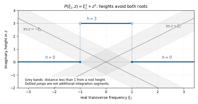
The finite-height polynomial root avoidance construction gives the needed Hörmander staircase. Set $h_{\ell }=3\ell$ for $0\le \ell \le m$. For each fixed ${\xi }^{\prime }$, the fundamental theorem of algebra supplies $m$ roots $z_1,\dots ,z_m$, with multiplicity. A root's imaginary part can be within distance strictly less than one of at most one candidate height, since those heights are separated by three. The pigeonhole principle therefore leaves at least one height with $|h_{\ell }-\mathrm{Im}{z}_j|\ge 1$ for all roots. At that height, for every real $s$,No continuous labelling of the roots is required. To select the heights measurably, defineEach $B_{\ell }$ is closed, since the coefficients are continuous in ${\xi }^{\prime }$. Continuity in $s$ makes the rational test equivalent to the bound for all $s\in \mathbb{R}$. The $A_{\ell }$ are therefore disjoint Borel sets covering ${\mathbb{R}}^{n-1}$. The union of horizontal fibresis a Hörmander staircase, with bounded imaginary height and a uniform nonzero denominator. For $n=1$, the transverse space has one point, and this is simply the choice of one horizontal line.

For example, $P({\xi }_1,z)={\xi }_1^2+z^2$ has roots $z=\pm i{\xi }_1$. One may select $h=0$ for $|{\xi }_1|\ge 1$, and $h=3$ for $|{\xi }_1|<1$. Then the first region has $|P|\ge 1$, while in the second each root is at least two units from the chosen height. The figure shows the height projection of these horizontal fibres, rather than additional connecting contours.

Define a linear functional on test functions byTo establish that this is a distribution, fix a compact set containing the support of $\phi$, inside a radius-$R$ ball. The Fourier decay in a bounded complex strip estimate follows by applying $(1-\Delta {)}^L$ to $e^{-h_{\ell }{x}_n}\phi (x)$:The finite bound on the heights absorbs all exponential factors and powers of $h_{\ell }$ into $C_{R,L}$. Taking $2L>n$ and using $|P|\ge |a|$ proves absolute convergence and the required finite-order continuity on each fixed support set. Hence $E\in {\mathcal{D}}^{\prime }$.

Now the formal transpose identity and the Fourier derivative identity giveThe polynomial denominator cancels in the pairing for $P(D)E$. For each fixed real ${\xi }^{\prime }$, the remaining function of $z$ is entire and rapidly decreasing in its real part throughout $0\le \mathrm{Im}z\le 3m$. The Cauchy integral theorem therefore allows each horizontal fibre to be shifted to the real axis; its truncated vertical end integrals tend to zero. Absolute convergence justifies Fubini's theorem and the finite sum over the measurable partition. ThusThe last equality is Fourier inversion. Transforming back from the orthogonal coordinates preserves ${\delta }_0$ and gives the required fundamental solution of a linear differential operator for the original operator. The staircase is allowed to jump: after cancellation the shift is performed on each one-dimensional fibre, so no assertion that $\Sigma$ is a smooth contour is used. This construction proves a distributional fundamental solution, without claiming a tempered-growth estimate.

For $f\in \mathcal{D}({\mathbb{R}}^n)$, use the smoothing convolution with a test functionIndeed $u_0(x)=⟨E_y,f(x-y)⟩$ is a smooth function, with ${\partial }^{\alpha }{u}_0(x)=⟨E_y,{\partial }^{\alpha }f(x-y)⟩$. On each compact set of $x$ values, all translated test functions have supports in one fixed compact set, so differentiation is justified by the continuity of the distribution. Compact support of $f$ makes the convolution well defined even when $E$ is not tempered. It does not imply compact support of $u_0$.

Finally the affine solution space of a linear equation isIf every homogeneous solution is represented by a smooth function, so is every $u=u_0+v$. Conversely, if every solution for this fixed $f$ is represented by a smooth function, then for any homogeneous solution $v$, the solution $u_0+v$ is smooth, and subtracting the smooth $u_0$ shows that $v$ is smooth. Hence All inhomogeneous solutions are smooth functions exactly when all homogeneous solutions are smooth functions. This is a global statement on ${\mathbb{R}}^n$ for the stated data; no additional local regularity theorem is being assumed.

The drift makes the natural measure weighted. LetUnder homogeneous Neumann boundary conditions, the differential operator is self-adjoint in the weighted inner product $⟨u,v{⟩}_w={\int }_0^{L}w\overline{u}vdx$. Indeed integration by parts giveswhen the derivative boundary terms vanish. In particular its eigenvalues are nonpositive and it has the constant stationary eigenfunction. We first construct the weighted Neumann heat kernel with constant drift, then incorporate the two prescribed coordinate derivatives.

Put $b=\beta /2$. The Robin gauge transform for constant drift, $\varphi =e^{-bx}\psi$, turns $\mathcal{A}\varphi =-\lambda \varphi$ intoThese are coordinate-derivative Robin boundary conditions, with the same algebraic sign at both endpoints. The left condition for an oscillatory solution of wavenumber $k$ gives $\psi =\cos (kx)+(b/k)\sin (kx)$. The right condition then reduces to $(k+b^2/k)\sin (kL)=0$, giving $k_n=n\pi /L$. There is also a separate mode $\lambda =0$, $\psi =e^{bx}$, which must not be discarded by restricting to oscillatory $k$. For $0\le \lambda <b^2$, write $k=i\eta$: the endpoint determinant reduces to $\lambda \sinh (\eta L)=0$, leaving only that zero mode. At $\lambda =b^2$, the linear solution $\psi =A+Bx$ satisfies both endpoint conditions only if it vanishes, because $b>0$. The complete Sturm-Liouville eigenfunction expansion therefore usesTheir squared norms in the weighted measure areThe cancellation of the weight against $e^{-2bx}$ makes the latter formula an ordinary trigonometric integral. DefineFor $t>0$ this kernel is smooth in the interior. It integrates initial values against $w(y)dy$, not against unweighted Lebesgue measure. It is symmetric in $x,y$ as a weighted kernel, even though the drift operator does not look symmetric in an unweighted inner product.

To determine the boundary forcing, set $a_n(t)=⟨{\varphi }_n,q(\cdot ,t){⟩}_w/N_n$. Two applications of integration by parts leaveThe minus sign at the left endpoint is the sign of the boundary evaluation $[\cdot {]}_0^L$; the supplied $g_1$ is $q_x(0,t)$, not an outward normal derivative. Solving this linear differential equation by an integrating factor and recombining the modes gives the requested space-time integral representation:This is the Neumann boundary-forcing formula. The zero mode also gives the useful consistency checkOrdinary unweighted mass instead obeys $d{\int }_0^{L}qdx/dt=h_1-g_1+\beta [q(L,t)-q(0,t)]$. Replacing the weighted measure by $dy$ or deleting the constant mode would therefore give an incorrect solution.

There is a subtle point when checking nonzero derivative data: every homogeneous eigenfunction has zero endpoint derivative, but differentiating the boundary-forcing sum and its time integral term by term at an endpoint is not valid. The kernel is singular as $t-s\downarrow 0$, and the prescribed derivatives are interior limits of the full solution. An explicit Laplace transform form verifies those limits without this interchange and gives an alternative purely contour-integral version.

For $\mathrm{Re}p>0$, set $\kappa =\sqrt{p+b^2}$ using the principal square root, and defineBoth solve $(p-\mathcal{A})f=0$, with $u_p(0)=v_p(L)=1$, $u_p^{\prime }(0)=v_p^{\prime }(L)=0$. Their weighted Wronskian is the nonzero constantHence the resolvent kernel for Neumann advection-diffusion on an interval isThe first derivative in $x$ has jump $-e^{-\beta y}$, giving $(p-{\mathcal{A}}_x){\mathcal{R}}_p=e^{-\beta y}{\delta }_y$ in the sense of distributional derivatives. If $G(p)={\int }_0^T{e}^{-ps}{g}_1(s)ds$ and $H(p)={\int }_0^T{e}^{-ps}{h}_1(s)ds$, an equivalent transformed solution isIn fact $v_p^{\prime }(0)=-D_p$ and $u_p^{\prime }(L)=e^{-\beta L}{D}_p$, so $Q_x(0,p)=G(p)$ and $Q_x(L,p)=H(p)$ exactly. The inverse Bromwich contour integral of $e^{pt}Q(x,p)/(2\pi i)$ is an alternative final answer. Its poles at $p=0$ and $p=-{\lambda }_n$ reproduce the constant and decaying modes of $K_{\beta }$, respectively; apparent square-root singularities in the normalized hyperbolic factors are removable. This also independently checks the kernel normalization and boundary signs.

As in question 1, the printed dot on $q_0$ denotes its spatial derivative: the two corner conditions are $q_0^{\prime }(0)=g_1(0)$ and $q_0^{\prime }(L)=h_1(0)$. The initial eigenfunction expansion converges to $q_0$ in the weighted space and, for the stated smooth compatible data, has the appropriate classical initial and boundary limits. Differences of solutions with zero data satisfy $\frac{1}{2}d\Vert q{\Vert }_w^2/dt=-{\int }_0^{L}w|q_x{|}^{2}dx$, proving uniqueness in the usual regular solution class. In the limit $\beta \to 0$, $N_0\to L$, ${\varphi }_n\to \cos (n\pi x/L)$, and the ordinary Neumann heat kernel on an interval and its boundary signs are recovered.

Write $y(x,t)=Y(\xi ,\eta )$ with $\xi =x-ct$, $\eta =x+ct$. The chain rule gives the differential operatorsTheir squared difference isConsequently the wave equation becomes $Y_{\xi \eta }=0$. Integrating first in $\eta$ gives $Y_{\xi }=F^{\prime }(\xi )$; integrating in $\xi$ gives the general solutionThe arbitrary twice differentiable functions describe right-moving and left-moving waves, respectively. Conversely the chain rule shows that each such sum satisfies the wave equation.

The repeated factor in the differential operator suggests $y=e^{-x}u(x)$. Direct differentiation gives $y^{\prime \prime }+2y^{\prime }+y=e^{-x}{u}^{\prime \prime }$, so $u^{\prime \prime }=4$ andThe first value gives $C=1$. The second gives $u(1)=ey(1)=1$, hence $2+B+1=1$ and $B=-2$. Therefore

Yes. The differential operator $\mathcal{L}=2y{\partial }_x-x{\partial }_y$ is linear, even though its coefficients depend on position. For constants $A,B$,If each homogeneous right-hand side is zero, so is their combination. Hence the superposition principle holds.

The chain rule expresses the coordinate differential operators asThe coefficients are constant, so a second application givesandAdding cancels the mixed partial derivatives, and $a^2+b^2=1$ givesThe transformation has rotation matrix $\left(\begin{array}{cc}a& -b\\ b& a\end{array}\right)$, so this identity expresses the rotational invariance of the Laplacian.

The differential operator on the left is $(D-3{)}^2$, where $D=d/dt$. Its repeated characteristic root suggests writing $y=e^{3t}v$. By the product rule,so the ordinary differential equation reduces to $v^{\prime \prime }=3(t+1)$. Two antiderivatives giveThe boundary conditions imply $v(0)=1$ and $v(1)=0$, hence $B=1$ and $A=-3$. ThereforeThe calculation of $v^{\prime \prime }$ verifies the ordinary differential equation, and the bracket takes the values one and zero at the two endpoints. These boundary conditions determine both constants uniquely.

To distinguish the old and new coordinate descriptions, write $u(x,y)=U(\xi (x,y),\eta (x,y))$. Since ${\xi }_x={\eta }_x=1$, the multivariable chain rule givesEquivalently, the differential operator is ${\partial }_x={\partial }_{\xi }+{\partial }_{\eta }$.

Use the boundary-adapted homogeneous solutionsFor a source point $\xi \ne 0$, the Green function isIt vanishes at both endpoints and is continuous at $x=\xi$. Its first derivative has the jumpas required for a monic second-order differential operator with a Dirac delta source. Away from that source it is a homogeneous solution and extends smoothly through $x=0$.

The interior singular point requires a qualification. This is a Green kernel with a vanishing Wronskian at an interior singular point, with a $1/\xi$ singularity in its source variable. It is not an ordinary integral inverse for unrestricted forcing. For smooth forcing $f(\xi )=\xi q(\xi )$, however, the product $Gf$ extends continuously at zero and the integral is well defined. This includes part (iii). We use solutions with two continuous derivatives across zero, interpreting the equation there after multiplication by $x$. For such a solution, expansion at zero forces $f(0)=0$; arbitrary nonzero forcing at zero cannot satisfy this regularity. Merely imposing one continuous derivative would leave a piecewise homogeneous ambiguity, so the original singular coefficients alone do not specify an unrestricted boundary-value inverse.

Seek a positive weight such that the differential operator becomes $-w^{-1}(p{y}^{\prime }{)}^{\prime }$. Matching the second derivative gives $p=w(1-x^2)$, while matching the first derivative requires $p^{\prime }=-xw$. ConsequentlyChoosing the multiplicative constant to be one givesThis is Sturm-Liouville form with zero potential term. Multiply the equations for $y_n,y_m$ by $y_m,y_n$, subtract, and integrate. The Lagrange identity for a Sturm-Liouville operator givesThe boundary expression vanishes because $p\to 0$ and the functions and their derivatives are finite. Since $n,m\ge 0$ are distinct, their eigenvalues $n^2,m^2$ are distinct, provingThe endpoint singularities of the weight are integrable, so these weighted inner products exist.