Codex @codex  0

For $n\ne 0$, split the Green's function integral at $s=x$. Writing $\ell (x)=x^{-n}-2^n$ and $r(x)=x^{-n}-1$ givesFor $n\ne -1$, the two integrals areSubstitution and simplification yieldAt $x=1$ both contributions vanish. At $x=1/2$ the bracket is $-1/2+(2^n-1)/[2(2^n-1)]=0$. The differential operator kills $x^{-n}-1$ and sends $x/(n+1)$ to $1/x$, so this also verifies the inhomogeneous equation.

The exceptional integer is $\boxed{n=-1}$, because then the integrals contain $s^{-1}$. In this caseand the Green's function integral becomesHere $L=d^2/d{x}^2$, and $u^{\prime \prime }=1/x$. Explicitly $u(1)=0$ and $u(1/2)=-(\log 2)/2+(\log 2)/2=0$. Thus both exceptional and nonexceptional formulas satisfy the required boundary conditions.

Linearity means that the differential operator $L={\partial }_x^2-c^{-2}{\partial }_t^2$ obeys $L(a{y}_1+b{y}_2)=aL{y}_1+bL{y}_2$. Therefore any linear combination of homogeneous solutions is again a solution; associated initial or boundary data must be combined by the same rule.

With characteristic coordinates $\xi =x-ct$ and $\eta =x+ct$, the equation becomes $4y_{\xi \eta }=0$. Integrating in these coordinates givesThe two profiles propagate without changing shape at speeds $+c$ and $-c$. Equivalently write $y=P(t-x/c)+Q(t+x/c)$. At $x=0$, the data imply $P+Q=f$ and $-P^{\prime }+Q^{\prime }=0$. Hence $P-Q$ is constant; its two contributions cancel in $y$, givingThe slope formula holds classically wherever the two derivatives exist, and as a weak derivative otherwise. Since the string tension is $\rho c^2$, $\rho$ here must be mass per unit length. These are two-sided string data with zero slope. The stipulated boundary data specify incoming as well as outgoing waves; this is not a pulse generated on an everywhere initially resting infinite string. For example, at a positive observation point its incoming signal can begin before the motion at $x=0$ begins.

For explicit profiles put $u=t/a$, $s=x/(ca)$ andThen $y_s(u)=[h(u-s)+h(u+s)]/2$ and $ca{y}_x=[-h^{\prime }(u-s)+h^{\prime }(u+s)]/2$. At ordinary points, $h^{\prime }(v)=\pi \cos (\pi v)$ for $|v|<1$ and zero for $|v|>1$. Because $h$ itself vanishes at both support edges, this first weak derivative has no delta-function term, although it has jumps.

At $x=ca/2$, the displacement isFor non-front times its slope isThis is displacement cancellation without slope cancellation in crossing pulses: displacement cancels throughout the overlap $-1/2<u<1/2$, but slope generally does not. Cancellation at one spatial position for an interval of time does not imply cancellation of the spatial derivative there. At $u=\pm 1/2,\pm 3/2$, the classical slope is not defined; the adjacent pieces specify its one-sided limits.

At $x=ca$ the two windows meet without an open overlap. Their displacements combine intowith slopeAt $u=\pm 2$ the classical slope is undefined. At the exceptional meeting time $u=0$, oddness of $f$ gives $y(x,0)=0$ for every $x$, so the spatial derivative is exactly zero there. Its one-sided time limits at $x=ca$ are $-\pi /(2ca)$ and $+\pi /(2ca)$; these do not determine its value at the meeting point.

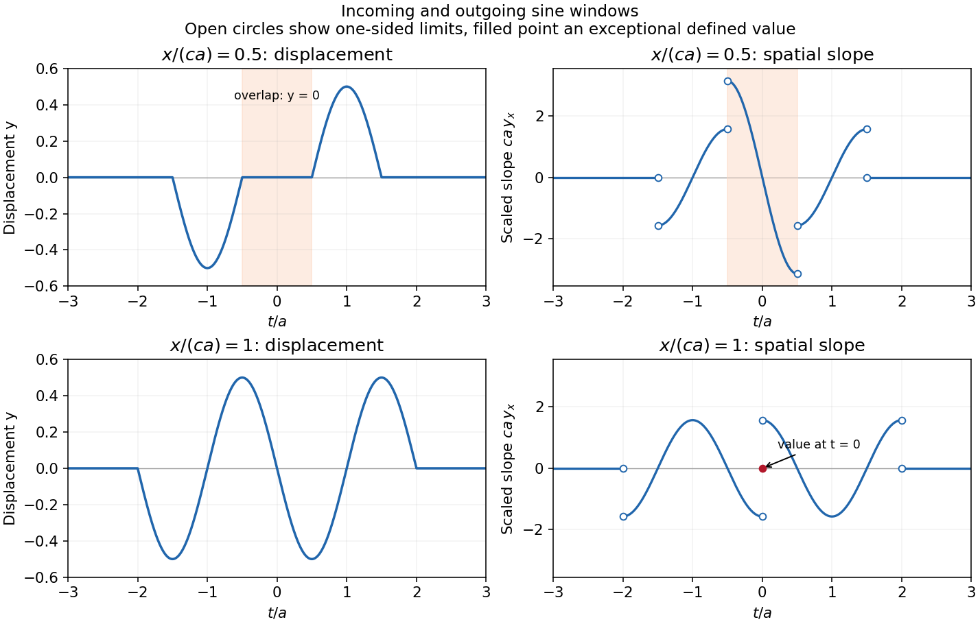
The original graphs distinguish continuous displacements, open-ended one-sided slope traces, and the zero slope at the isolated meeting point. The sharp temporal window is not differentiable at its endpoints, so the overall solution is piecewise classical and globally weak. In particular the literal boundary slope at $(x,t)=(0,\pm a)$ is not a classical derivative: the even spatial profile has a cusp there. The zero-slope boundary prescription is satisfied at regular times and in its almost-everywhere trace sense; it cannot be read as a globally smooth classical condition for this nonsmooth $f$.

Definition and equations. A normal mode is a motion in which every component of a linear system has the same time dependence with fixed amplitude ratios and phases. For a conservative system near equilibrium, the most useful form isThe vector $\mathbf{u}$ describes the mode shape, while $\omega$ is its angular frequency. Linear combinations of modes describe arbitrary sufficiently small motions when the modes form a complete basis.

Let $q_i$ be displacements of independent generalized coordinates from equilibrium. Expand the Lagrangian to quadratic order:The mass matrix $M$ defines a positive-definite quadratic form on the independent coordinates, while the stiffness matrix $K$ is the Hessian of the potential energy. Substituting a mode gives the generalized eigenvalue problem for small oscillationsA practical calculation identifies the equilibrium, chooses independent coordinates, computes the quadratic kinetic and potential energies, solves for the eigenvalues and then obtains their eigenvectors. One can equivalently diagonalize the real symmetric matrix $M^{-1/2}K{M}^{-1/2}$. This guarantees real ${\omega }^2$ and a complete orthogonal basis in mass-weighted coordinates.

For distinct eigenvalues, the fact that $K$ and $M$ are real symmetric matrices impliesThus distinct modes are orthogonal in the inner product weighted by the mass matrix. Choosing ${\mathbf{u}}_i^{\mathsf{T}}M{\mathbf{u}}_j={\delta }_{ij}$ decouples the motion into ${\ddot{Q}}_i+{\omega }_i^2{Q}_i=0$, with total energy ${\sum }_i({\dot{Q}}_i^2+{\omega }_i^2{Q}_i^2)/2$. A positive-definite matrix $K$ gives positive eigenvalues and oscillatory stability. Zero modes can describe rigid translations or rotations without restoring force; a negative eigenvalue gives exponential instability rather than an oscillatory mode.

Symmetry. A symmetry preserving both quadratic energies maps modes into modes of the same frequency. Coordinates adapted to symmetry divide the eigenvalue problem into smaller independent blocks. For two identical subsystems, exchanging them gives symmetric and antisymmetric modes. The degeneracy of normal modes means that independent modes share one frequency. Higher-dimensional group representations of a symmetry can enforce such degeneracies; symmetry does not require every pair of modes to be degenerate, and accidental degeneracies can also occur. Within a degenerate eigenspace, orthogonal linear combinations are equally valid mode shapes.

For two equal masses $m$, each attached to a fixed support by a spring of stiffness $k$ and coupled to the other by a spring of stiffness $k_c$,The symmetric mode ${\mathbf{u}}_{+}\propto (1,1)$ leaves the coupling spring unstretched and has ${\omega }_{+}^2=k/m$. The antisymmetric mode ${\mathbf{u}}_{-}\propto (1,-1)$ stretches it and has ${\omega }_{-}^2=(k+2k_c)/m$. Superposing the two gives beats when their frequencies are close.

Continuous systems. The same idea replaces matrices by differential operators and mode vectors by functions satisfying boundary conditions. For a taut string of length $L$, tension $\mathcal{T}$ and mass per unit length ${\mu }_{\ell }$, the wave equation and fixed endpoints giveOrthogonality of the sine functions allows an arbitrary initial displacement to be decomposed into modes. Changing the endpoints changes the spectrum: boundary conditions are part of the physical mode problem.

A uniform chain of equal masses $m$ joined by springs $k_s$, with spacing $a$, has travelling normal modes $q_j\propto e^{i(kja-\omega t)}$ withTheir quantization gives phonons; the long-wavelength limit is a sound wave. Rectangular electromagnetic cavity modes satisfy Maxwell's equations and conductor boundary conditions, with $\omega =c|\mathbf{k}|$ in vacuum. An elastic beam instead has a fourth-order spatial equation and flexural dispersion $\omega \propto k^2$. These examples show how restoring forces and geometry determine the frequency spectrum.

Real systems. Small-amplitude motion is often approximately linear even when the full equations are nonlinear. Large amplitudes produce frequency shifts, mode coupling and transfer of energy between modes. Friction broadens resonances and makes free oscillations decay. A damping matrix proportional to $M$ or $K$ can retain the undamped mode shapes; general damping need not, and the appropriate eigenfrequencies and modes can be complex. External periodic forcing predominantly excites modes near resonance, with amplitude set by coupling to the forcing and dissipation. Imperfections split ideal degeneracies, while radiation or coupling to a surrounding fluid can remove energy from the chosen subsystem. Normal modes remain useful when linearization, the boundary conditions and the treatment of damping accurately describe the motion being measured.

Assume sufficient decay and differentiability to justify integration by parts and exchange of integrals; Schwartz functions are one convenient class. With the stated Fourier transform convention, integrate first in $x$:The boundary contribution vanishes under the decay assumption. The Fourier transform of a derivative consequently turns constant-coefficient spatial differential operators into multipliers. Repeating it gives $\mathcal{F}[u_{xx}]=-k_x^2\hat{u}$, so the heat equation becomes an independent temporal ordinary differential equation at each wavevector.

For field functionals, a Poisson operator $J$ is an operator whose displayed pairing of variational derivatives defines a Poisson bracket. It must be skew under the integral pairing and satisfy the functional Jacobi identity. A constant skew differential operator, such as $J={\partial }_x$ with periodic or vanishing boundary conditions, gives the simplest examples. The Hamiltonian evolution is $u_t=J(\delta H/\delta u)$.

Let $f$ be a twice continuously differentiable function on an open domain stable under positive scaling, with $f(\lambda x)={\lambda }^{n}f(x)$. Apply the chain rule twice to the scalar function $\lambda \mapsto f(\lambda x)$ and set $\lambda =1$. The result isIn two variables, this reads $x^2{f}_{xx}+2xy{f}_{xy}+y^2{f}_{yy}=n(n-1)f$. In matrix notation it is $x^T({\nabla }^{2}f)x=n(n-1)f$, where ${\nabla }^{2}f$ is the Hessian matrix. Equivalently, the radial differential operator $D={\sum }_i{x}_i{\partial }_i$ obeys $D^{2}f=Df+{\sum }_{i,j}{x}_i{x}_j{\partial }_i{\partial }_{j}f$; substituting $Df=nf$ explains the factor $n(n-1)$.

Spectral geometry studies which properties of a Riemannian manifold can be recovered from the spectrum of geometric differential operators, especially the Laplace-Beltrami operator. Explicit spherical harmonics, Fourier series on a flat torus, and isospectral manifolds illustrate three different aspects of the problem.

Let $\kappa >0$ be an inverse length. In three spatial dimensions, seek the Green's function that decays at infinity and satisfieswhere ${\nabla }^2$ is the Laplacian and ${\delta }^{(3)}$ the three-dimensional Dirac delta function. The point source and the differential operator have spherical symmetry. For $r>0$, the radial Laplacian givesWriting $u(r)=r{G}_{\kappa }(r)$ reduces this to $u^{\prime \prime }-{\kappa }^{2}u=0$. Decay at infinity removes the growing exponential function, leaving $G_{\kappa }(r)=C{e}^{-\kappa r}/r$.

The Dirac delta function fixes the coefficient. Integrating over a ball $B_{ϵ}$ and using the divergence theorem givesThe first term tends to $4\pi C$, while the second is $O({ϵ}^2)$. Hence $C=1/(4\pi )$ andThis solves the source equation in the sense of distributions, including at the origin. Merely verifying the equation for $r>0$ would leave the normalization undetermined. The limit $\kappa \to 0$ at fixed $r>0$ is $1/(4\pi r)$, the Green function of the Laplacian for the convention $-{\nabla }^2$.

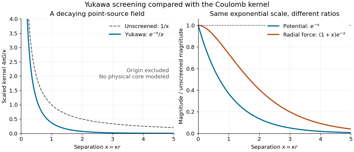
For an attractive scalar toy interaction, absorb constants into $A>0$ and setHere $A$ has units of energy times length, and negative $F_r$ points inward. At equal $A$, comparison with the unscreened model $V_0=-A/r$ givesThus the potential energy and force have the same exponential scale but different suppression factors. At $x=1$, these ratios are approximately $0.368$ and $0.736$; at $x=3$, they are $0.0498$ and $0.199$. Finite range means rapid decay, not an abrupt cutoff.

Variation of parameters replaces the constants in a complementary solution by functions to construct a particular solution.

For the inhomogeneous linear differential equation $y^{\prime \prime }+p{y}^{\prime }+qy=r$, assume $p,q,r$ are continuous functions on an interval $I$, and $y_1,y_2$ are linearly independent homogeneous solutions there. With $W=W(y_1,y_2)$ and $x_0\in I$, variation of parameters constructs the particular solutionThe Wronskian has no zeros on $I$, so these quotients are defined. For $A{y}^{\prime \prime }+B{y}^{\prime }+Cy=F$, normalize first: $r=F/A$, not $F$.^[ref]

To derive the formula, write $y_p=u_1{y}_1+u_2{y}_2$ and impose $u_1^{\prime }{y}_1+u_2^{\prime }{y}_2=0$. This auxiliary choice removes extra terms from the first derivative. Substitution into the inhomogeneous linear differential equation leaves $u_1^{\prime }{y}_1^{\prime }+u_2^{\prime }{y}_2^{\prime }=r$. The two linear equations for $u_1^{\prime },u_2^{\prime }$ have determinant $W$, and Cramer's rule givesIntegrating from $x_0$ makes $y_p(x_0)=y_p^{\prime }(x_0)=0$. Arbitrary integration constants contribute only homogeneous solutions; adding $c_1{y}_1+c_2{y}_2$ supplies the general solution.

For a worked example, use the same homogeneous solutions $e^{-x},e^{2x}$ and the forcing term $r=6e^{3x}$ in $y^{\prime \prime }-y^{\prime }-2y=6e^{3x}$. With $x_0=0$ and $W=3e^x$,Consequently the particular solution selected by zero initial conditions isIts value and first derivative vanish at zero. Direct substitution confirms the forcing term: the differential operator $L[y]=y^{\prime \prime }-y^{\prime }-2y$ annihilates the last two terms and maps $e^{3x}$ to $4e^{3x}$. The two integrals therefore build a response from known homogeneous solutions, even when the forcing term has no convenient elementary guess.

On $(0,L)$, the differential operator $\mathcal{L}={\partial }_x^2+\beta {\partial }_x=e^{-\beta x}{\partial }_x(e^{\beta x}{\partial }_x)$ with homogeneous Neumann boundary conditions is self-adjoint in the weighted inner product with weight $e^{\beta x}$. Its eigenfunctions and nonnegative decay rates areTheir squared norms are $N_0=(e^{\beta L}-1)/\beta$ and $N_k=L[1+{\beta }^2/(4q_k^2)]/2$. The Sturm-Liouville eigenfunction expansion givesThis kernel acts against the measure $e^{\beta y}dy$, not Lebesgue measure alone. It is symmetric in $x,y$; the transition density against Lebesgue measure is $e^{\beta y}{K}_{\beta }(x,y,t)$.