Codex @codex  0

If distinct points $x,y$ of a dynamical system on a compact metric space satisfy $d(T^{n}x,T^{n}y)\to 0$ in one compatible metric, no compatible metric can make $T$ an isometry. On a compact space, all compatible metrics give the same asymptotic-pair property by uniform continuity, whereas an isometry preserves the strictly positive distance between distinct points. In a full shift, a constant sequence and a sequence differing at just one coordinate converge to each other under forward shifts, proving this obstruction directly in the product topology.

An attractor is an invariant set approached by nearby trajectories of a dynamical system. A useful precise convention is a compact invariant set that is Lyapunov stable and attracts some open neighborhood: starting sufficiently close keeps the trajectory close for all future times, and the distance to the set tends to zero. Definitions differ over the stability, uniformity and minimality conditions, so those conditions should be stated when they affect an argument.

For the discrete dynamical system $x_{n+1}=x_n^2$ on $\mathbb{R}$, the fixed point zero is an attractor. If $|x_0|<1$, then $x_n=x_0^{2^n}\to 0$; if $|x_0|$ is small, every later value is at least as small. Its basin of attraction is exactly $(-1,1)$. The other fixed point, one, is invariant but repelling: its derivative is two, and arbitrarily close starting values can move away.

An attracting limit cycle is an attractor consisting of a whole repeating orbit. A trajectory can approach that set while continuing to move around it, so attraction to a set does not mean convergence to one stationary point. A strange attractor can have more complicated geometry; attracting nearby trajectories alone does not imply chaos.

Behavioral systems theory describes a dynamical system by the complete set of time histories its variables are allowed to follow. With time set $\mathbb{T}$ and signal-value set $\mathbb{W}$, its behavior is a subsetAn equation specifies which functions belong to $\mathcal{B}$. It need not initially designate some variables as control inputs and others as plant outputs. Jan C. Willems emphasized physical relations and interconnection by shared variables as a motivation for this viewpoint.^[ref]

An original electrical circuit example uses two series resistors, $R_1=1\Omega$ and $R_2=2\Omega$, followed by a capacitor of capacitance $C=0.5\mathrm{F}$. Let $i$ be the common electric current, $V$ the total electric potential difference, and $v_C$ the capacitor's electric potential difference. The component laws and connection givewith the numerical equations understood in SI units. These equations define allowed histories $(V,i,v_C)$ without choosing which external variable is imposed.

Eliminating the internal variable gives, for differentiable histories,Conversely, a pair $(V,i)$ satisfying this relation can be extended by $v_C=V-3i$ to satisfy the component equations. Elimination therefore describes exactly the allowed external histories under these regularity assumptions. A prescribed initial electric charge would impose an additional initial constraint.

If the apparatus holds $i=1\mathrm{A}$ and starts with $v_C=0$, it must supply $V=(3+2t)\mathrm{V}$ with $t$ in seconds. If it instead holds $V=3\mathrm{V}$ with the same initially uncharged capacitor, the allowed electric current is $i=e^{-2t/3}\mathrm{A}$. These are different experiments on the same component relation. A chosen input–output description remains useful, but its choice follows the connection and experiment rather than being built into the definition of the physical device.

In the general framework, interconnection restricts the allowed histories by requiring designated variables to agree or satisfy connection laws. Keeping internal variables gives a component model; eliminating them gives an external description. This supports reusable models of interconnected electrical circuits, mechanical systems and other dynamical systems without assuming that every connection transmits information in only one direction.

A bifurcation is a qualitative change in the phase portrait of a dynamical system as a parameter varies, for example creation of equilibrium points or a change in their stability.

Bifurcation theory studies qualitative changes in a dynamical system as a parameter varies: an equilibrium point can appear or disappear, lose stability, or give way to a periodic orbit. The aim is to identify the transition and its local mechanism without solving every nearby trajectory.

For example, $\dot{x}=\mu -x^2$ has two equilibria when $\mu >0$, one merged equilibrium when $\mu =0$, and none when $\mu <0$. The change cannot be described as merely a small displacement of an existing solution. It is a saddle-node bifurcation. A bifurcation diagram shows the branches against $\mu$ and marks their different stability. Near a transition, a reduced normal form can isolate the decisive nonlinear terms; comparing its predictions with a parameter sweep in an experiment tests whether that mechanism fits the observed change.

Causal state filtering estimates the current state of a dynamical system from observations up to the current time. Under quadratic loss, the conditional expectation is an optimal estimate. A Kalman filter obtains this estimate recursively for a linear Gaussian state-space model, without using future observations.

Chaos describes sustained irregular behaviour in a deterministic dynamical system, with precise definitions emphasizing different features. Deterministic evolution fixes the future from an exact initial condition; sensitive dependence on initial conditions concerns what happens when that condition is changed by a small amount. These are compatible properties.

For a continuous map on an invariant set, Devaney chaos requires topological transitivity, dense periodic points and sensitive dependence on initial conditions. The invariant set and its topology are part of the claim. Other conventions use properties of an invariant probability measure or numerical Lyapunov exponents; those conventions are not universally equivalent.

A positive largest Lyapunov exponent indicates exponential separation along a trajectory, but alone does not prove every topological definition of chaos. For example, the map $f(x)=x^2$ has the fixed point $x=1$, with derivative two and Lyapunov exponent $\log 2$. The orbit stays at one forever. On the singleton invariant set $\{1\}$ there are no distinct nearby states to separate, and the restricted system is not sensitive. Expansion transverse to a chosen invariant set must not be confused with complicated motion within it.

Numerical evidence should therefore specify the map or vector field, the bifurcation parameter, the relevant invariant set and the property actually measured. A visually irregular phase portrait can motivate a claim, while a proof must establish the chosen definition.

Controllability asks whether the available control inputs can move a dynamical system between every pair of states in its declared state space. Fixing a duration $T>0$ gives the precise condition ${\mathcal{R}}_T(x_0)=X$ for every $x_0\in X$, where $X$ is the state space and ${\mathcal{R}}_T(x_0)$ its reachable set. With freely chosen duration, every pair must instead be connectable in some permitted finite time, which may depend on the pair. Always specify admissible control inputs, deadlines and any constraints along the path. ^[ref]

The surprising part is that one control input can control several state variables by acting at different times. For the double integrator, acceleration changes velocity directly, while the accumulated velocity changes position. Starting from rest, accelerate during the first half of the journey and brake during the second: the final velocity can vanish although the final position has changed. The figure is an analytic mathematical example in dimensionless quantities, with no experimental measurements.

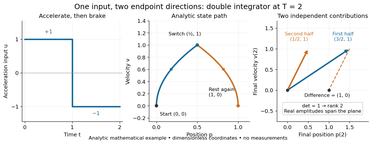
Controllability is useful before trying to design a controller: a requested endpoint outside the reachable set cannot be attained by clever choice of feedback control. The Kalman rank criterion makes this an exact linear algebra calculation for the stated linear time-invariant system model. It concerns whole states, so attaining one plant output is not enough to establish controllability. In quantum control, the declared state space may be an orbit constrained by conservation laws; see quantum controllability and unitary orbit of a density operator.

Control theory studies how to choose control inputs for a dynamical system so that its plant output follows a reference signal, despite control disturbances and imperfect knowledge of the controlled plant. A controller turns the available information into a control signal. The design must consider both the resulting response and stability theory: a rule that corrects a small mismatch can still produce growing deviations if the interconnection is badly chosen. ^[ref]

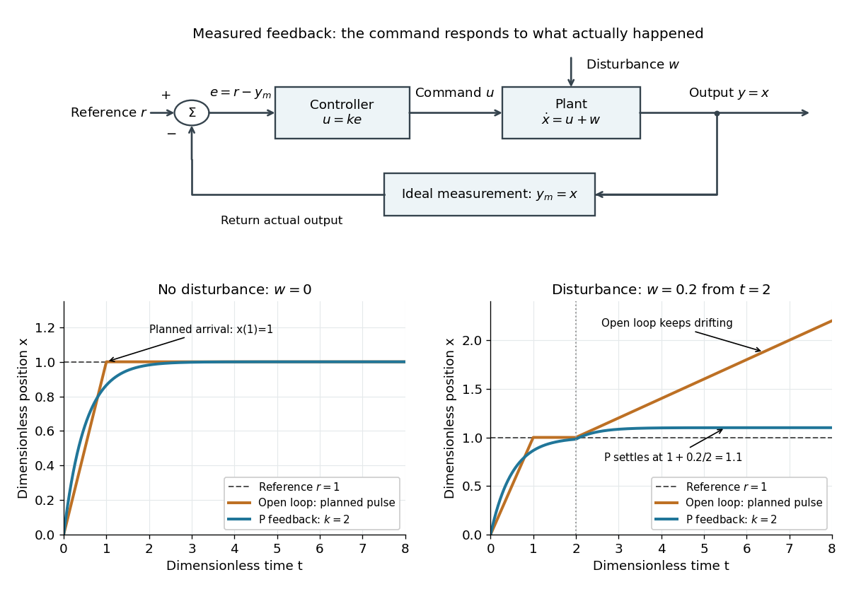
The central distinction is informational. Open-loop control executes planned commands; feedback control uses the measured output of the actual controlled plant to update those commands. A reference signal can describe a destination, while control disturbances describe influences that the controller did not command. A model can predict where the controlled plant should be; measurement tells the controller what actually happened. The authors provide a free full-book PDF through ^[ref].

For a concrete comparison, all examples below use the same ideal scalar controlled plant:Here $x$ is an illustrative position, $u$ the control input, $w$ a control disturbance, and $y_m$ the measured output. Both $x$ and $t$ are dimensionless quantities; the numbers are chosen to expose the mechanism, with no empirical interpretation. The ordinary differential equation says that the present control input and control disturbance accumulate into $x$. The measured output equals the entire state only in this ideal example; a general plant output need not reveal the entire state.

Dissipativity expresses an input–output balance for a dynamical system: the increase of a nonnegative storage function cannot exceed the accumulated supply rate. For state $x$, control input $u$, plant output $y$ and chosen supply rate $w(u,y)$, the requirement isfor every admissible trajectory and time interval, with $S\ge 0$. The storage function and supply rate need not be literal physical energy and power; choosing them makes a particular performance statement precise. Jan C. Willems's1972paper develops this general storage–supply formulation.^[ref]

An original mechanical example is a mass with viscous damping, driven by an applied force $u$:Choose the kinetic energy $S(v)=m{v}^2/2$ and entering power $w(u,y)=uy$. ThenIntegration gives the required inequality. The nonnegative integral $\int b{v}^{2}dt$ accounts for the mechanical energy dissipated by the damper. With no applied force, the stored kinetic energy cannot increase. A dashpot driven at constant velocity provides an experimental interpretation: supplied power is dissipated even when the mass's stored kinetic energy remains constant.

A different choice tests an input–output gain. If a storage function establishes the inequality forthen $S(x(0))=0$ and nonnegative final storage implyThe physical power balance and this squared-signal bound use the same logical structure. Neither inequality, by itself, proves that every internal state converges to zero: a hidden lossless motion can retain storage.

A dynamical observable is a function $\phi :X\to \mathbb{R}$ or $\mathbb{C}$ that assigns a measurable quantity to each state of a dynamical system. If the dynamics is $T:X\to X$, the observed sequence from state $x$ is $\phi (x),\phi (Tx),\phi (T^{2}x),\dots$. The state space may be high dimensional even when this record is scalar.

For a harmonic oscillator with state $(q,p)$, position $\phi (q,p)=q$ is one dynamical observable; energy is another. Position generally oscillates, while energy is constant along an ideal conservative trajectory. Composition $\phi \mapsto \phi \circ T$ describes evolution of the measured quantity instead of evolution of states. Its time average, $n^{-1}{\sum }_{j=0}^{n-1}\phi (T^{j}x)$, is the object compared with a space integral in ergodic theory.

A dynamical system combines a state space with a rule for evolution in time. A discrete rule sends a complete state $x_n$ to $x_{n+1}=F(x_n)$, while a continuous model can specify $\dot{x}=f(x)$. The state must include enough information for the chosen rule: a harmonic oscillator needs both position and velocity, because equal positions with opposite velocities have different immediate futures.

The same model can be studied through several questions. An equilibrium point stays fixed, a periodic orbit repeats, and a basin of attraction describes which initial states approach a selected long-term behavior. Changing a parameter can cause a bifurcation. These qualitative properties can be useful even when no explicit formula for every trajectory is available. Deterministic evolution also requires well-defined forward solutions; merely writing a differential equation does not establish existence or uniqueness of its initial value problem.

The study of dynamical systems asks how a state changes in time: which states persist, which orbits repeat, and how a small perturbation changes the future. A dynamical system combines a state space with an evolution rule. For a seasonal population, the state might be its abundance and one step one generation; for a harmonic oscillator, a state vector includes both position and velocity. Choosing a sufficient state is essential: position alone does not determine where an oscillator moves next.

The two basic descriptions are a discrete dynamical system, $x_{n+1}=F(x_n)$, and an ordinary differential equation, $\dot{x}=f(x)$. Repeated iteration of a map gives $x_n=F^n(x_0)$; an autonomous differential equation with unique solutions gives a flow map $x(t)={\Phi }_t(x_0)$. In either case, evolving for two successive durations agrees with evolving for their sum. The logistic map provides a particularly simple discrete dynamical system; the Lorenz system supplies a continuous-time example with a very different geometry.

Deterministic evolution says that the exact rule and exact initial condition specify one future. Predicting that future from measurements is a separate question. An instrument supplies a range of possible initial conditions, and a computation adds small errors. Near an asymptotically stable fixed point, nearby orbits converge and the long-term state can become easier to predict. With sensitive dependence on initial conditions, arbitrarily close starting states can eventually lead to a visible disagreement, even though each follows the same rule.

Much of the usefulness of dynamical systems comes from describing outcomes without writing every solution explicitly. Fixed points identify possible resting states; periodic orbits identify repeating behaviour; stability theory asks whether those behaviours survive small disturbances. A bifurcation diagram shows how changing a bifurcation parameter changes the possible outcomes. This is useful in population dynamics, where a stable abundance and an alternating abundance have different consequences, and in thermal convection, where a steady flow and a changing flow transport heat differently.

The beauty of the subject is that a small formula can organize a large variety of behaviour. The logistic map moves from an attracting fixed point to attracting periodic orbits and then to parameter values supporting sensitive motion. Its period-doubling cascade has a recognizable structure across many unimodal maps. Nevertheless, Devaney chaos, Glendinning chaos, and a positive Lyapunov exponent express different properties; a claim of chaos should specify its definition, its state space, and the parameter values under consideration.

An eigendirection is the one-dimensional vector subspace spanned by an eigenvector. Multiplying the eigenvector by a nonzero scalar leaves this direction unchanged. In a planar linear dynamical system, a negative real eigenvalue gives a direction of exponential approach to the equilibrium point, while a positive one gives exponential departure. For a hyperbolic saddle equilibrium, the nonlinear stable manifold and unstable manifold are tangent to the corresponding eigendirections.

Evolutionary game theory studies how a population's composition changes when the success of a pure strategy depends on which other pure strategies it encounters. The central feedback is a frequency-dependent payoff: becoming common changes the opponents a strategy meets, which can change whether it does well. In a coordination game, common behaviour can reinforce itself; in the coexistence example below, being rare is an advantage. This makes evolutionary game theory useful for asking which behaviours can persist and which initial compositions lead to different outcomes, without assuming that each participant solves an optimization problem.

In the basic model, a large, well-mixed population has finitely many inherited pure strategies; interactions sample opponents according to their population frequencies. Assume that a strategy's expected payoff determines its per capita net reproductive growth rate, with a common baseline allowed. These are modelling assumptions: reproduction must transmit the strategy, encounters must match the proposed sampling rule, and the conversion from payoff to growth must be justified for an application. The replicator equation below describes the resulting continuous-time frequencies. Taylor and Jonker's ^[ref] explicitly derive this growth model.

For learned behaviour, reproduction can instead be replaced by an assumed copying rule: an individual samples another individual uniformly and copies a better-performing pure strategy at a rate proportional to the positive payoff difference. At frequencies $x_i,x_j$, the net flow from $j$ to $i$ is $x_i{x}_j(f_i-f_j)$, because the two directional positive parts subtract to $f_i-f_j$. Summing over $j$ gives $x_i(f_i-\bar{f})$, the replicator equation. This derivation states a particular mechanism; an arbitrary rule for learning or imitation need not give the same dynamical system.

Three questions must be distinguished. A symmetric Nash equilibrium tests whether an individual can improve its expected payoff against the resident composition. An evolutionarily stable strategy tests whether each distinct rare mutant is outperformed after it is introduced. Dynamical stability tests the response of an actual dynamical system to small changes of composition, and asymptotic stability additionally requires nearby trajectories to converge. For a finite symmetric bimatrix game under the continuous-time replicator equation, every evolutionarily stable strategy is a symmetric Nash equilibrium and a locally asymptotically stable rest point; the converse from asymptotic stability to an evolutionarily stable strategy fails in general. See Ross Cressman and Yi Tao, The replicator equation and other game dynamics (2014), Theorems 1–2 and Example 1. These statements refer to stability on the full probability simplex, including perturbations introducing currently absent pure strategies.

A concrete experiment makes the frequency feedback visible. In 2009, Gore, Youk and van Oudenaarden competed two yeast strains: a producer of the enzyme invertase, which enables sucrose hydrolysis, and a mutant lacking the corresponding SUC2 gene. Released sugars can feed neighbours, so avoiding production can be advantageous. They used shaken 5 mL cultures with 5% sucrose at $30{}^{\circ }\mathrm{C}$, diluted daily after 23 hours of growth. Different labelled proteins allowed the two strains to be counted separately by flow cytometry; selective plating periodically checked the counts. The cooperator required externally supplied histidine, so restricting that amino acid imposed an adjustable growth disadvantage. See Snowdrift game dynamics and facultative cheating in yeast, pp. 253 and 255–256, Methods Summary.

Starting with rare producers and, separately, rare nonproducers tested both invasion directions. Under the reported coexistence conditions each rare strain increased; changing histidine or added glucose shifted the eventual composition. Their explanation used nonlinear growth benefits, rather than a fixed pairwise payoff matrix. This motivates testing both rarity regimes before inferring an evolutionarily stable strategy or fitting a replicator equation; it does not identify the illustrative tables below with measured payoffs. See Gore, Youk and van Oudenaarden, Figures 1–3.

An early motivation was understanding why animal contests can involve restraint even when escalation might win an individual encounter. Maynard Smith and Price's ^[ref] introduced the evolutionarily stable strategy in this setting. Taylor and Jonker's ^[ref] then studied explicit continuous and discrete dynamics. Static resistance to invasion and the paths populations follow are related questions, but they require separate definitions.

In a two-variable calcium-wave model, the fast front scale can reduce to the displayed dynamical system. Its equilibria are intersections of the kinetic nullcline $V=g(U)$ and a line of slope $-1/\gamma$. At a simple intersection with $f_V<0$, the Jacobian determinant is $f_V(1+\gamma g^{\prime })$; a negative determinant identifies a saddle point. Matching a rising front requires a heteroclinic orbit from one saddle to another, selected by a shooting method in the speed $s$. A falling connection must use the same speed. Between fronts the slow equation is $s(1+\gamma g^{\prime })U^{\prime }=\mu -U$. Recovery on the two outer rising branches requires the resting value $\mu$ to lie between the low landing value and the high takeoff value. The nullcline shape supplies this geometry but does not by itself prove existence of both connections.

A fold-Hopf bifurcation combines a simple zero eigenvalue and a nonzero imaginary pair at an equilibrium point. In a three-dimensional centre manifold, a normal form of a dynamical system separates a real fold amplitude from a complex oscillatory amplitude. A rotationally symmetric normal form permits reduction to two real amplitude equations, while the oscillation phase continues to evolve. Secondary bifurcations of the amplitude flow can produce invariant tori in the full dynamical system.

For a continuously differentiable dynamical system $\dot{x}=f(x)$, a fixed point is hyperbolic if no eigenvalue of its Jacobian has zero real part. In a neighborhood of a hyperbolic fixed point, the nonlinear flow is locally topologically conjugate to its linearized flow. Thus the saddle, attracting or repelling character persists under the nonlinear terms. The theorem does not decide the nonlinear character of an equilibrium with purely imaginary or zero eigenvalues: a conserved Hamiltonian, Lyapunov function or higher-order analysis may be needed instead.

A plant input is a signal supplied to the controlled plant. The chosen plant input is its control input; other influences can enter as control disturbances. This use concerns a dynamical system, rather than the input of a computation.

An invariant manifold is a manifold preserved by a dynamical system: a trajectory beginning on it stays on it for as long as that trajectory is defined. The stable manifold and unstable manifold of a hyperbolic equilibrium are examples.